1.1.9. Physics Picture¶

1.1.9.1. Rabi oscillations¶

Hamiltonian of Rabi oscillation is

\[\begin{split}H = -\frac{\omega_m}{2} \begin{pmatrix} 1 & 0 \\ 0 & -1 \end{pmatrix} - A \cos(k t)\begin{pmatrix} 0 & 1 \\ 1 & 0 \end{pmatrix} .\end{split}\]

The Hamiltonian we could solve is

\[\begin{split}H &= -\frac{\omega_m}{2} \sigma_3 - \frac{A}{2} \begin{pmatrix}0 & e^{i k x} \\ e^{-i k x} & 0 \end{pmatrix} \\ & = -\frac{\omega_m}{2} \sigma_3 - \frac{A}{2} \cos(kx) \sigma_1 + \frac{A}{2} \sin (kx) \sigma_2 ,\end{split}\]

which has a transition probability

\[P(x) = \frac{\lvert A\rvert^2}{ \lvert A\rvert^2 + (k - \omega_m)^2 } \sin^2 \left( \sqrt{ \lvert A\rvert^2 + (k - \omega_m)^2 } x/2 \right).\]

With two perturbations

\[H' = -\frac{\omega_m}{2} \sigma_3 - \frac{1}{2} (A_1 \cos(k_1 x) + A_2 \cos(k_2 x)) \sigma_1 + \frac{1}{2}( A_1 \sin (k_1x) + A_2 \sin (k_2 x) ) \sigma_2.\]

If \(k_1 \gg k_2\), we can approximate by treating the slow rotating perturbation as a constant added to the energy gap, so that the new energy gap is shifted

\[\omega_m' = \sqrt{ \omega_m^2 + A_2^2 },\]

which could possibly shift the system out of resonance.

The best practice would be applying this to the different modes.

1.1.9.2. Oscillations and Modes¶

Using Jacobi-Anger expansion, for any system with Hamiltonian

\[H = -\frac{\omega_m}{2} \sigma_3 + \frac{1}{2}\sum_n A_n \sin (k_n x) \cos 2\theta_m \sigma_3 - \frac{1}{2}\sum_n A_n \sin (k_n x) \sin 2\theta_m \sigma_1,\]

we could rewrite the system into a composition of multiple Rabi oscillations

\[\begin{split}H = -\frac{\omega_m}{2} \sigma_3 + \frac{1}{2} \sum_{n_1} \cdots \sum_{n_N} \begin{pmatrix} 0 & B_{n_1,\cdots,n_N} \Phi_{n_1,\cdots, n_N} e^{i \left( \sum_{a} n_a k_a \right)x} \\ B_{n_1,\cdots,n_N}^* \Phi_{n_1,\cdots, n_N}^* e^{-i \left( \sum_{a} n_a k_a \right)x} & 0 \end{pmatrix}.\end{split}\]

For each mode, we have a Rabi oscillation

\[\begin{split}H_{n_1,\cdots,n_N} = -\frac{\omega_m}{2} \sigma_3 + \frac{1}{2} \lvert B_{n_1,\cdots,n_N} \rvert \begin{pmatrix} 0 & e^{i \left( \sum_{a} n_a k_a \right)x} \\ e^{-i \left( \sum_{a} n_a k_a \right)x} & 0 \end{pmatrix},\end{split}\]

where we have dropped \(\Phi_{n_1,\cdots, n_N}\) and the possible sign and phase of \(B_{n_1,\cdots,n_N}\) since these phase terms only determines the phase of the perturbation on xy plane.

To explain the interference, we explore the superposition of two modes,

\[\begin{split}H \equiv -\frac{\omega_m}{2} \sigma_3 + \frac{1}{2} \lvert B_1 \rvert \begin{pmatrix} 0 & e^{i \left( \sum_{a} n_a k_a \right)x} \\ e^{-i \left( \sum_{a} n_a k_a \right)x} & 0 \end{pmatrix} + \frac{1}{2} \lvert B_2 \rvert \begin{pmatrix} 0 & e^{i \left( \sum_{a} n_a' k_a \right)x} \\ e^{-i \left( \sum_{a} n_a' k_a \right)x} & 0 \end{pmatrix},\end{split}\]

which is composed of two Rabi oscillations. We choose the first mode to be the one close to resonance, i.e., \(\sum_a n_a k_a \sim \omega_m\), while the second mode is far away from resonance.

For simplicity we use two perturbations, that is \(a=1,2\). The Hamiltonian can be written as

\[H = -\frac{\omega_m}{2} \sigma_3 + \frac{1}{2} ( \lvert B_1\rvert \cos(\phi_1 x) + \lvert B_1 \rvert \cos (\phi_2 x) )\sigma_1 - \frac{1}{2} ( \lvert B_1 \rvert \sin (\phi_1 x) + \lvert B_2 \rvert \sin(\phi_2x) ) \sigma_2,\]

where we define \(\phi_1 = n_1 k_1 + n_2 k_2\) and \(\phi_2 = n_1' k_1 + n_2' k_2\). Using Pauli matrices are basis, this corresponds to a Hamilton vector

\[\begin{split}\vec H = \begin{pmatrix} - \lvert B_1\rvert \cos(\phi_1 x) - \lvert B_2 \rvert \cos (\phi_2 x) \\ \lvert B_1 \rvert \sin (\phi_1 x) + \lvert B_2 \rvert \sin(\phi_2x) \\ \omega_m \end{pmatrix} = \begin{pmatrix} 0 \\ 0 \\ \omega_m \end{pmatrix} + \begin{pmatrix} - \lvert B_1\rvert \cos(\phi_1 x) \\ \lvert B_1 \rvert \sin (\phi_1 x) \\ 0 \end{pmatrix} + \begin{pmatrix} - \lvert B_2 \rvert \cos (\phi_2 x) \\ \lvert B_2 \rvert \sin(\phi_2x) \\ 0 \end{pmatrix},\end{split}\]

which has a z component and two rotating perturbations. We choose the system to be

\[\begin{split}\phi_1 &\sim \omega_m \\ \phi_2 & \neq \omega_m.\end{split}\]

We then have two different situations, \(\phi_2/\omega_m \gg 1\) and \(\phi_2/\omega_m \ll 1\).

1.1.9.2.1. Slow Perturbation¶

For \(\phi_2/\omega_m \ll 1\), the second mode is a very slow rotating perturbation, which can be explained using the proposed theory.

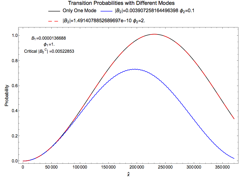
../../_images/rabi-oscillation-interference-of-different-modes.png — Fig. 1.36 Resonance interference of modes. The combination of the first mode and \(B_2=\)¶

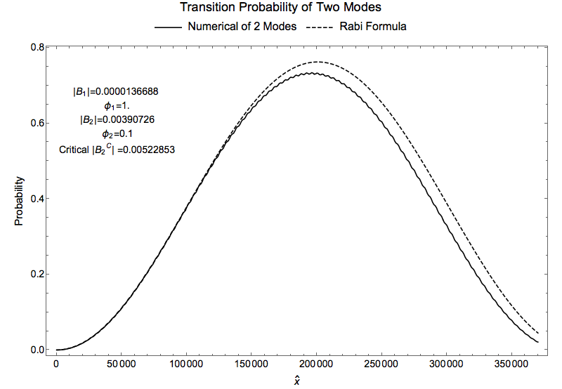
../../_images/rabi-oscillation-interference-of-different-modes-compare-rabi-formula.png — Fig. 1.37 Compare with Rabi formula¶

As a test of the theory, we can calculate the ratio of each \(B_2\), which depends on the modes, and the critical value \(B_2^C\) which is the crtical value for the destruction of the resonance.

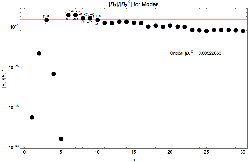
../../_images/rabi-oscillation-interference-of-different-modes-b2-over-b2critical.png — Fig. 1.38 Ratio \(\lvert B_2\rvert/\lvert B_2^C \rvert\)¶

To summarize, in the modes view, resonance of some modes are destroyed by some certain modes.

1.1.9.3. Example of Full System¶

First we choose a system that is on resonance

\[H_1 = -\frac{\omega_m}{2} \sigma_3 + \frac{\delta \lambda_1}{2} \cos 2\theta_m \sigma_3 - \frac{\delta \lambda_1}{2} \sin 2\theta_m \sigma_1,\]

where \(\delta\lambda_1 = A_1 \sin (k_1 x)\), where \(k_1 = \omega_m\) and \(A_1 = 3.5\times 10^{-5}\omega_m\). This sets the system to resonance.

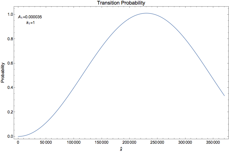
../../_images/resonance-freq-example-1.png — Fig. 1.39 Resonance¶

Does the Diagonal Term Matter?

Removing the diagonal elements of the perturbation

\[H_1' = -\frac{\omega_m}{2} \sigma_3 - \frac{\delta \lambda_1}{2} \sin 2\theta_m \sigma_1,\]

will result in Fig. 1.40.

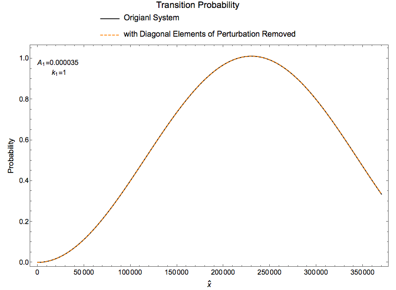
../../_images/resonance-freq-example-1-compare-with-diagonal-elements-of-perturbation-removed.png — Fig. 1.40 Remove the diagonal elements of the preturbation¶

Adding in Slowly Changing Field

Add a new slow perturbation

\[\delta \lambda_2 = A_2 \sin (k_2 x),\]

with

\[\begin{split}A_2 &= 10^{-2},\\ k_2 &= 0.1.\end{split}\]

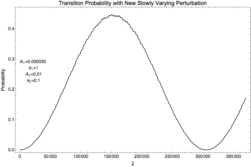
../../_images/resonance-freq-example-1-added-new-slow-perturbation.png — Fig. 1.41 Added new slow perturbation¶

Removing Diagonal Elements of Slow Perturbation

Removing the diagonal elements of slow perturbation

\[H_2' = -\frac{\omega_m}{2} \sigma_3 + \frac{\delta \lambda_1 }{2} \cos 2\theta_m \sigma_3 - \frac{\delta \lambda_1 + \delta \lambda_2}{2} \sin 2\theta_m \sigma_1,\]

gives us the result Fig. 1.42.

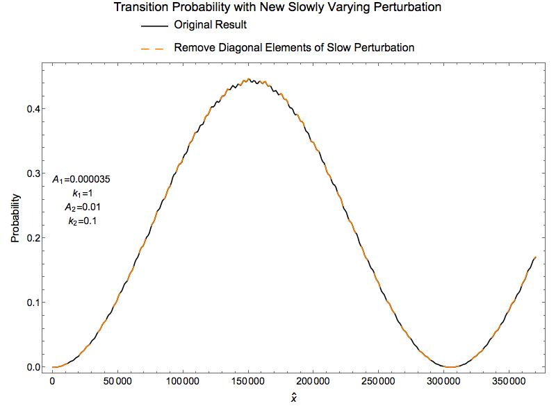
../../_images/resonance-freq-example-1-added-new-slow-perturbation-compare-with-removing-diagonal-elements.png — Fig. 1.42 Remove diagonal elements of slow perturbation.¶

1.1.9.4. Explaination¶

Slow perturbation is slow and changes the energy gap of the system. Since the energy gap \(\omega_m\) determines the resonance point, which is

\[k_1 = \omega_m,\]

adding the slow perturbation could increase \(\omega_m\),

(1.27)¶\[\begin{split}\omega_m' &= \sqrt{A_{2,\bot} ^2 + \omega_m^2} \\ & = \omega_m \sqrt{ \left(\frac{A_{2,\bot}}{\omega_m} \right)^2 + 1 } \\ & \approx \omega_m + \frac{A_{2,\bot}^2}{2\omega_m},\end{split}\]

where \(A_{2,\bot}\) is component perpendicular to z axis.

Only Perpendicular Component

In the calculation of the modified energy gap, we used only the perpendicular component of the new slow perturbation. This only holds for \(A_{2,\bot} \ll \omega_m\).

PROOF

Shift The System Out of Resonance

Shift the system out of resonance, it is required that

\[\lvert \omega_m' - k_1 \rvert \gtrsim \text{width of resonance} A_1.\]

Width of resonance is basically determined by \(A_{1,\bot}\). Apply equation (1.27), we can solve the condition to break the resonance,

\[A_{2,\bot} \gtrsim \sqrt{2\omega_m A_{1,\bot}}.\]

In our example, the condition becomes

\[\begin{split}&A_2 \sin 2\theta_m \gtrsim \sqrt{2\omega_m A_1 \sin 2\theta_m} \\ \Rightarrow & A_2 \gtrsim \sqrt{2\omega_m A_1 \tan 2\theta_m/\cos 2\theta_m}.\end{split}\]

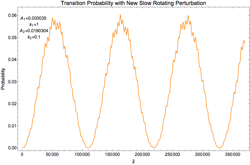
../../_images/resonance-freq-example-1-added-new-slow-perturbation-destruction.png — Fig. 1.43 With \(A_2=\sqrt{2 A_1 \sin (2 \theta_m)}/ \cos ^2(2 \theta_m) =0.0190304\omega_m\)¶

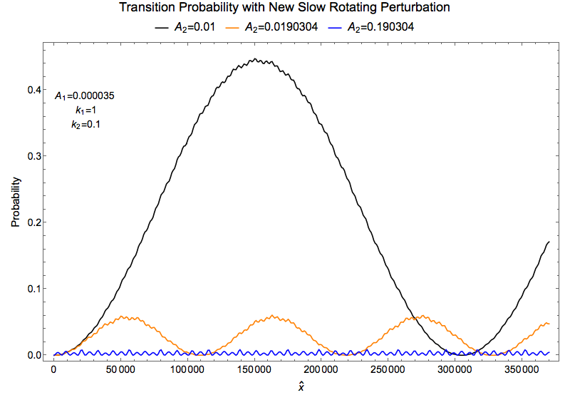
../../_images/resonance-freq-example-1-added-new-slow-perturbation-destruction-compare.png — Fig. 1.44 Compare to show destruction¶

Using Rabi formula the amplitudes are not matching the numerical calculations, Fig. 1.45.

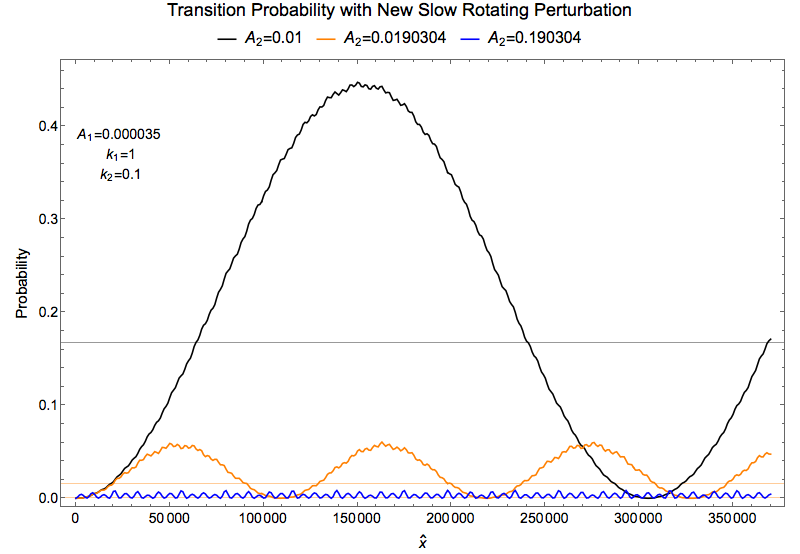
../../_images/resonance-freq-example-1-added-new-slow-perturbation-destruction-compare-gridlines.png — Fig. 1.45 Grid lines are the amplitudes predicted by Rabi formula.¶

As a reference, the Q values for each line are

\[\begin{split}Q_1 & = \frac{\lvert k_1 - \sqrt{A_2 \sin^2(2\theta_m) + 1 } }{A_1\sin (2\theta_m)} = 1.11689, \\ Q_2 & = \frac{\lvert k_1 - \sqrt{A_2' \sin^2(2\theta_m) + 1 } }{A_1\sin (2\theta_m)} = 4.04469, \\ Q_3 & = \frac{\lvert k_1 - \sqrt{A_2'' \sin^2(2\theta_m) + 1 } }{A_1\sin (2\theta_m)} = 402.277.\end{split}\]

However, the important question is whether the modified oscillation really Rabi oscillation. The answer is NO.

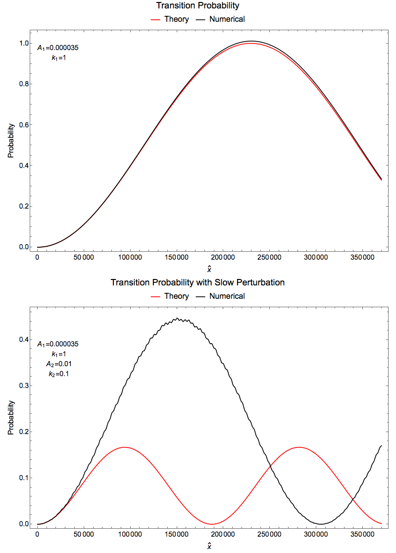
../../_images/really-rabi-question-mark.png — Fig. 1.46 Is the oscillation with slow perturbation really Rabi oscillation? Upper panel: Theoretical and numerical calculation of original system; Lower panel: Theoretical and numerical calculation with slow perturbation added.¶

We can not predict the oscillation when we add in the new perturbation using the Rabi oscillation formula. That makes sense!

1.1.9.4.1. Introducing Another Component Perturbation¶

We add in the term that has two components,

\[H = - \frac{\omega_m}{2} \sigma_3 + \frac{\delta \lambda(x)}{2} \cos 2\theta_m \sigma_3 - \frac{\delta \lambda(x)}{2} \sin 2\theta_m \sigma_1 + \frac{\delta \lambda(x)}{2} \sin 2\theta_m \sigma_2.\]

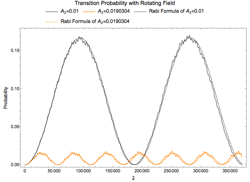
../../_images/resonance-freq-example-1-added-new-slow-perturbation-destruction-compare-rotating-field.png — Fig. 1.47 Add another component xy plane¶

1.1.9.4.2. Rotating Perturbation with Constant Strength¶

Construct a system with a mode at resonance and another rotating perturbation of constant length,

\[H = - \frac{\omega_m}{2} \sigma_3 - \frac{1}{2} (A_1\cos(k_1x) + A_2 \sin(k_2x)) \sigma_1 + \frac{1}{2} ( A_1\sin (k_1 x) + A_2 \sin(k_2 x) ) \sigma_2,\]

where we choose \(k_1\gg k_2\).

The new \(\sigma_2\) term is a rotating field with constant length, which makes sure the modified energy gap has a constant length rather than the slowly changing energy gap.

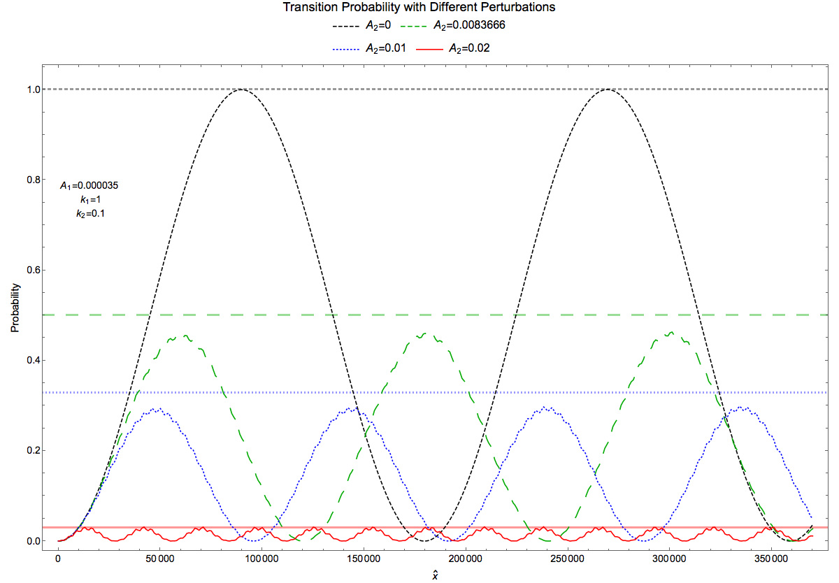
../../_images/rabi-oscillations-energy-gap-change.png — Fig. 1.48 Reduction of transition amplitudes. Black dashed line: one perturbation at exact resonance; Green long dashed line: \(A_2=A_{2,\mathrm{Critical}}=0.0083666\); Blue dotted line: \(A_2=0.01\); Red line: \(A_2=0.02\). The grid lines are the amplitude predicted using Rabi formula correspondingly.¶