7.6. Linear Stability Analysis
Reading List
Banerjee, A., Dighe, A., & Raffelt, G. (2011). Linearized flavor-stability analysis of dense neutrino streams. Physical Review D - Particles, Fields, Gravitation and Cosmology, 84(5), 1–19.
Raffelt, G., Sarikas, S., & Seixas, D. D. S. (2013). Axial Symmetry Breaking in Self-Induced Flavor Conversionof Supernova Neutrino Fluxes. Physical Review Letters, 111(9), 91101.
Izaguirre, I., Raffelt, G., & Tamborra, I. (2017). Fast Pairwise Conversion of Supernova Neutrinos: A Dispersion Relation Approach. Physical Review Letters, 118(2), 21101.
7.6.1. Some General Discussion
Tips about Matrices
Here are some conclusions about matrices.
Skew symmetric = anti-symmetric.
Eigenvalues of symmetric matrix are real.
Eigenvalues of skew-symmetric matrix are either 0 or imaginary.
7.6.2. First Approach
For some references, please read [chakraborty2016].
The conventions used in [chakraborty2016] are
Equation of motion:
\[i(\partial_t + \mathbf v^{(i)} \cdot \mathbf\nabla)\rho^{(i)} = [ H^{(i)},\rho^{(i)} ].\]Linearized density matrix
(7.2)¶\[\begin{split}\rho = \frac{1}{2}\begin{pmatrix} 1 & \epsilon \\ \epsilon^* & -1 \end{pmatrix}.\end{split}\]In general, the density matrix can be decomposed into trace part and traceless part,
\[\begin{split}\rho = \frac{1}{2}\mathrm{Tr}(\rho) \boldsymbol{I} + \frac{1}{2}\begin{pmatrix} a-\mathrm{Tr}(\rho) & \epsilon \\ \epsilon^* & (1-a)-\mathrm{Tr}(\rho) \end{pmatrix}.\end{split}\]The trace part is a constant, thus we drop it and redefine the density matrix as the traceless part.
\[\begin{split}\rho = \frac{1}{2}\begin{pmatrix} a & \epsilon \\ \epsilon^* & -a \end{pmatrix},\end{split}\]where \(a=1\) if we start from all electron flavor.
The fact that the number densities are different for different beams could be included in the density matrix or the coefficient in fron of it. In the paper by Chakraborty, Hansen, Izaguirre, and Raffelt [chakraborty2016] they include this difference in densities in the density matrix, which I find not so intuitive. So I would choose to define the density matrix similar to the single particle ones and define
\[\alpha\mu = \sqrt{2}G_F \alpha n_{\nu},\]where \(\alpha\) accounts for the differences in the densities for each beam.
The commutator of a general traceless Hamiltonian
\[\begin{split}H = \begin{pmatrix} -h_0 & h \\ h^* & h_0 \end{pmatrix}\end{split}\]and density matrix Eq. (7.2) is
\[\begin{split}[H,\rho] = \frac{1}{2}\begin{pmatrix} -h \epsilon^* + \epsilon h^* & 2h + 2 \epsilon h_0 \\ -2 h_0 \epsilon^* - 2 h^* & h \epsilon^* - \epsilon h^* \end{pmatrix}.\end{split}\]Thus the linearized equation for the perturbation for beam i is
(7.3)¶\[i(\partial_t+\mathbf v^{(i)}\cdot \boldsymbol \nabla) \epsilon^{(i)} = 2h^{(i)} + 2 \epsilon^{(i)} h_0^{(i)}.\]We only need to find \(h_0^{(i)}\) and \(h^{(i)}\) for each beam.
With the equation of motion (7.3), we would like to Fourier transform it
where \(Q(\Omega,\mathbf k)\) becomes the functions we need to solve, since the equation is linear to \(\epsilon\). To be specific,
where \(\mathbf A^{(i)}_{ij}\) is the coupling matrix due to \(h\). For example,
means
- chakraborty2016(1,2,3)
Chakraborty, S., Hansen, R. S., Izaguirre, I., & Raffelt, G. (2016). Self-induced neutrino flavor conversion without flavor mixing, (10), 17.
7.6.3. Second Approach
In this approach, we use conventions of the following.
Linearized density matrix
\[\begin{split}\rho = \begin{pmatrix} 1 & \epsilon \\ \epsilon^* & 0 \end{pmatrix}\end{split}\]Equation of motion without time de
7.6.3.1. Linearize the EoM
To linear the EoM we start from a state where almost all neutrinos are in one flavor,
Suppose we have a Hamiltonian in flavor basis of the form
the commutator of Hamiltonian and density matrix is
Mathematica Code
(* Define the density matrices and Hamiltonians *)
rho={
{1,epsilon},
{Conjugate@epsilon,0}
};
rhodiag={
{1/2,epsilon},
{Conjugate@epsilon,-1/2}
};
hamil={
{h1,h},
{Conjugate@h,h2}
};
hamil2={
{-h1,h},
{Conjugate@h,h2}
};

(* Calculate the Commutators *)

hamil.rho-rho.hamil//Simplify

{{h Conjugate[epsilon] - epsilon Conjugate[h], -h + epsilon (h1 - h2)}, {(-h1 + h2) Conjugate[epsilon] + Conjugate[h], -h Conjugate[epsilon] + epsilon Conjugate[h]}}

hamil2.rho-rho.hamil2//Simplify

{{h Conjugate[epsilon] - epsilon Conjugate[h], -h - epsilon (h1 + h2)}, {(h1 + h2) Conjugate[epsilon] + Conjugate[h], -h Conjugate[epsilon] + epsilon Conjugate[h]}}

hamil.rhodiag-rhodiag.hamil//Simplify

{{h Conjugate[epsilon] - epsilon Conjugate[h], -h +epsilon (h1 - h2)}, {(-h1 + h2) Conjugate[epsilon] + Conjugate[h], -h Conjugate[epsilon] + epsilon Conjugate[h]}}
We linearize the equation by keeping only the first order terms of \(\delta\). For this purpose, we need to calculate the neutrino self-interaction \(H_{\nu\nu}\).
However, from the general form of \(H_{\nu\nu}\), which is an integral or convolution of \(\rho\), we would expect that the off diagonal element of the Hamiltonian \(h\), is of first order, if we start from a density matrix that has first order, which is what we do. Thus we expect \(h \delta^*\) is second order effect, which we will neglect.
Finally, we obtain one equation for each beam, which can either be the (1,2) element or the (2,1) element.
7.6.3.2. Four-Beam Line Model
Some Definitions
We define some parameters in this section.
\(\eta\) is determines the hierarchy of the neutrinos. \(\eta=+1\) means normal hierarchy, and \(\eta=-1\) means inverted hierarchy. \(\beta\) takes care of the sign for the vacuum term and self-interaction term. For the vacuum term, \(\beta=(-)1\) for (anti)neutrinos. For the self-interaction term, \(\beta=(-)1\) if the beam is interacting with (anti)neutrinos.
We use \({}^L\) to denote the beam on the left, \({}^R\) to denote the beam on the right, and \(\bar{\epsilon}\) to denote that the beam is composed of anti-neutrinos.
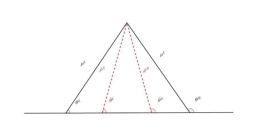
Fig. 7.7 Four beams model
For any line model of finite beams, we can specify each beam by three parameters,
where \(\rho\) is the density matrix of the beam, \(\theta\) is the angle of the beam defined by some rule, \(\alpha\) is the ratio of the particle number density to the neutrino number density. If we are talking about a neutrino beam instead of an anti-neutrino beam, we have \(\alpha=1\).
In the four-beam case, we define the system using the following three lists of parameters,
where the \(\epsilon\)’s are used to construct the perturbed density matrix,
Perturbed Density Matrix
We are interested in flavor conversion. So we start from a state with one flavor, which renders the density matrix
However, as dynamics is our concern, we need to add the perturbation to investigate the stability
So we can now write down the equation of motion for the system with this perturbed density.
\(\epsilon\) as a vector
In fact, as we’ll derive the linearized equations, \(\delta\) is used as a vector
With all the definitions and conventions specified, we can write down the equation of motion without trouble, IN PRINCIPLE.
First of all, we find the Hamiltonian,
The neutrino self interaction term requires some elabration on it. We take the left neutrino beam as an example. It experiences interactions with three beams, \(\{\bar\rho^L, \bar\theta^L, \alpha\}\), \(\{\bar\rho^R, \bar\theta^R, \alpha\}\), as well as \(\{ \rho^R, \theta^R, 1\}\). So \(H_{\nu\nu}^L\) should have three terms,
This procedure works for all other beams. Or we can use the power of the ALMIGHTY Mathematica.
The equation of motion is reduced to one equation about \(\delta\)’s for each beam.
where \(h_1\), \(h_2\) are determined by both \(H_v\), \(H_m\), and the self-interaction term \(H_{\nu\nu}\). \(h\) is determined by the expression of \(H_{\nu\nu}\). Then we rewrite the equation into the form
where \(M\) is the coefficient matrix that generates the equations we previously derived. This procedure can be done by Mathematica.
Notice that we have the equation with r as the variable, which is not very convenient. Even we solve the equation, it is very hard to interpretate the solutions since r is different at the same height z. So we have to rewrite the equation into one with vertical height z as the variable using \(i\partial_r = i \sin \theta \partial_z + i \cos \theta \partial_x\). Be very careful with the sign of \(+ i \cos \theta \partial_x\). In the four beam case, we have
The equation for the perturbations becomes
Simplified?
Define the following quantities
The lineaized equation of motion can be written in a simplified form.
Suppose we have the neutrino and antineutrino beams in the same direction, i.e., \(\theta_1=\theta_2\), the term \(\chi_-\) becomes 0.
Mathematica Code
The Mathematica code that describes the matrix M’ in equation
is
transMatrix[eta_, mk_, mu_, alpha_, theta1_, theta2_, lambda_, omegav_: 0] := Module[{},

   (* theta1 for neutrinos, theta2 for antineutrinos *)

   {
   {lambda + mu - 2 alpha mu - eta omegav + mu Cos[2 theta1] +
       2 alpha mu Sin[theta1] Sin[theta2],
      alpha mu - alpha mu Cos[theta1 - theta2], -mu -
       mu Cos[2 theta1], alpha mu + alpha mu Cos[theta1 + theta2]}/
     Sin[theta1] + mk Cot[theta1] {1, 0, 0, 0},
   {-mu + mu Cos[theta1] Cos[theta2] + mu Sin[theta1] Sin[theta2],
      lambda + 2 mu - alpha mu + eta omegav -
       alpha mu Cos[2 theta2] - 2 mu Sin[theta1] Sin[theta2], -mu -
       mu Cos[theta1] Cos[theta2] + mu Sin[theta1] Sin[theta2],
      alpha mu + alpha mu Cos[2 theta2]}/Sin[theta2] +
   mk Cot[theta2] {0, 1, 0, 0},
   {-mu - mu Cos[2 theta1],
      alpha mu + alpha mu Cos[theta1] Cos[theta2] -
       alpha mu Sin[theta1] Sin[theta2],
      lambda + mu - 2 alpha mu - eta omegav + mu Cos[2 theta1] +
       2 alpha mu Sin[theta1] Sin[theta2],
      alpha mu - alpha mu Cos[theta1] Cos[theta2] -
       alpha mu Sin[theta1] Sin[theta2]}/Sin[theta1] -
   mk Cot[theta1] {0, 0, 1, 0},
   {-mu - mu Cos[theta1] Cos[theta2] + mu Sin[theta1] Sin[theta2],
      alpha mu + alpha mu Cos[2 theta2], -mu +
       mu Cos[theta1] Cos[theta2] + mu Sin[theta1] Sin[theta2],
      lambda + 2 mu - alpha mu + eta omegav -
       alpha mu Cos[2 theta2] - 2 mu Sin[theta1] Sin[theta2]}/
     Sin[theta2] - mk Cot[theta2] {0, 0, 0, 1}
   }
]
If we are using a model that is homogeneous in x direction, the derivative is gone. We assume the solution is of the form \(\epsilon = \epsilon_0 e^{i\Omega z}\). By put the assumption back into the equation we obtain
Linear stability analysis basically becomes finding the eigenvalues of matrix \(M\). A negative imaginary part in \(\Omega\) means the solution can grow exponentially.
Some Questions
Even if we assume homogenous in x direction, will it be stable under small perturbations? I guess it also is not that easy to say since the equation of motion in x direction is somewhat similar to the equation in z direction, we might have some instability in x direction.
Is there any interpretation of the solution as a function of r?
For this four-beam model, the eigenvalues can be found analytically by Mathematica, eventhough the solution is a bit tedious. We work out the example using unit of \(\omega_v\), i.e., \(\hat \lambda=\lambda/\omega_v\) and \(\hat\mu = \mu/\omega_v\).
7.6.3.3. Neutrino Line Model with Fourier Analysis
Neutrino line model is discussed in [duan2015]. We’ll follow the paper.
The equation of motion is
where Hamiltonian
We discuss the equilibrium case so that the time dependent part vanishes.
For the line model, we have only two directions \(x\) and \(z\), thus the density matrix depends on these two directions, i.e., \(\rho(x,z)\). Since all the neutrinos emitted from a line located at \(z=0\), we can Fourier decompose the density matrix \(\rho(x,z)\) in the x direction
where \(k_0\) is determined by the size of the line \(L\),
Equivalently, we can linearize the equation first then Fourier transform the perturbations. Both methods works.
7.6.3.3.1. Fourier Transform of Density Matrix
As we plug it back into the equation of motion, left hand side becomes
The vacuum Hamiltonian and matter Hamiltonian are
The neutrino-neutrino interaction becomes
where \(\beta^{j}\) indicates if the beam is neutrino or antineutrino,
To save keystroke we define
where \(n_\nu\) is the number density of the neutrinos.
So we can write down the equation of motion for each beam, using the decomposed density matrix. It’s easily noticed that the equation is not coupled between Fourier modes of the density matrix.
For simplicity, we first solve the four beams case, c.f. Fig. 7.7, with \(\bar n_{\nu} = \alpha n_{\nu}\). The equation of motion for neutrino beam i reads
Horizontal Speed \(v_x^i\)
Please notice that the horizontal speed \(v_x^i\) has a different sign for left beam and right beam.
We have all the modes decoupled from each other. However, the different beams are coupled to each other for the same mode. Thus the equations for mode \(m\) can be combined into a single matrix differential equation, which is tedious to write down.
To analyze the instability, we apply the tricks in linear stability analysis, and define the perturbed density matrice
The only unknow functions are \(\epsilon^i_m\) and \(\bar\epsilon^i_m\).
Useful Commutation Relations
With the perturbed form of density matrix, we have several simple commutation relations.
We analyze the four beams model which has only one left beam and one right beam for neutrinos and antineutrinos, with the same geometry shown in Fig. 7.7. The equation of motion calculated from the linearized density matrix is
For the purpose of linear stability analysis, one the off-diagonal elements are needed. The equations for the perturbations becomes
where we have unified the notation of \(\epsilon\) and \(\bar\epsilon\). For the four beams model, the equations can be written down explicitly in principle. However, we could imagine the space it’s gonna take.
For simplicity we consider the case \(\theta^L = \theta^R \equiv\theta\) and \(\alpha^L=\alpha^R\). We also have \(v_x^R=\bar v_x^R= -v_x^L= -\bar v_x^L \equiv -v_x\).
Then the equations becomes
For convinience we define
so that the equations are
We actually have a problem. What are those couplings between different modes? Are these couplings really first order?
7.6.3.3.2. Fourier Transform Perturbations
The other idea is to linearize the equations first then Fourier transform only the perturbations. The result for the equations of perturbations can be obtained directly from Eq. (7.6),
We linearize the equation first before Fourier decomposition is applied. The linearized equation is basically (7.4), with different notations. Then we Fourier transform the equations,
The reason we have no coupling between different modes is that linearized equation of motion is linear to all the perturbations.
Construct a vector
from which we develop the matrix equation
We define
This non-Hermitian ‘evolution’ matrix \(\Upsilon_m\) introduces many new features in the evolutions of the perturbations since the eigenvalues of it are not garanteed to be real. Any imaginary part of the eigenvalues of it will give us exponential increase.
Plus-Minus Modes
In the paper [duan2015] the authors introduced the definition
The vector of functions to be solve is
This is simply a transformation of the vector we have, i.e., Eq. (7.7). The transformation matrix is
so that
We can find the corresponding ‘Hamiltonian’ matrix for the new vector by applying
What I get is
which is the same as the form derived in the paper [duan2015].
We can easily find the eigenvalues for the matrix \(Uplison_m\) or \(\Lambda_m\). Any imaginary part (not real part because we have an extra i in the equation) of the eigenvalue will lead to exponential growth of the perturbations.
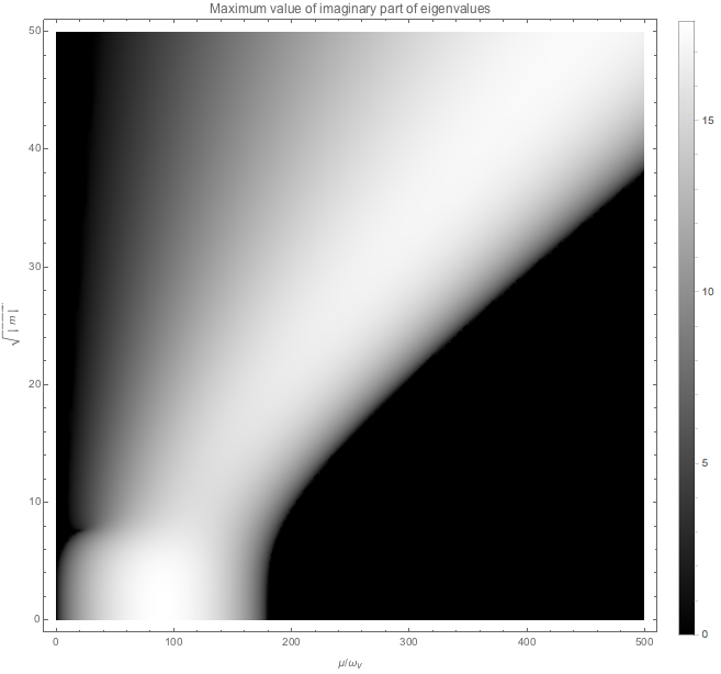
Fig. 7.8 Maximum of imaginary part of the eigenvalues of matrix \(\Upsilon_m\) for different \(\chi\) and \(m\). This amazing result says that larger neutrino density leads to the instability on smaller scales. This result is for \(\alpha=0.8\), \(v_z=1/2\), \(k_0=2\pi/L=2\pi/(20\pi/\omega_v)\), and \(\lambda=0\).
Eigenvalues of \(\Upsilon_m\) and \(\Lambda_m\) are the same
The reason is that the determinant of the following two matrice are the same,
since determinant has cyclic permutation symmetric.
We also notice that matter has no effect on this phenomenon because we can remove matter effect by minus a matrix \(\frac{1}{v_z}\lambda \mathbf I\) from matrix \(\Upsilon_m\), while the eigenvalues is not changed. What’s more important, the evolution of the perturbation doesn’t change under such a manipulation.
- duan2015(1,2,3)
Duan, H., & Shalgar, S. (2015). Flavor instabilities in the neutrino line model. Physics Letters, Section B: Nuclear, Elementary Particle and High-Energy Physics, 747, 139–143.