5.1. MSW Effect¶

Brief Summary of MSW Resonance

The Hamiltonian for matter effect is

\[\mathbf H(x) = \left(\frac{\lambda(x)}{2} -\frac{ \omega_{\mathrm{v}} }{2} \cos 2\theta_{\mathrm{v}}\right) \boldsymbol {\sigma_3 } + \frac{ \omega_{\mathrm{v}} }{2} \sin 2\theta_{\mathrm{v}} \boldsymbol{\sigma_1},\]

where \(\lambda(x)=\sqrt{2}G_F n_e(x)\) is the matter potential and \(\omega_{\mathrm{v}}=\frac{\Delta m^2}{2E}\) is the vacuum oscillation angular frequency. MSW resonance happens when the diagonal terms disappear, i.e.,

\[\lambda = \omega_{\mathrm{v}} \cos 2\theta_{\mathrm{v}}.\]

What does it mean?

Now think about the vacuum Hamiltonian in flavor basis,

\[\mathbf{H}_{\mathrm{vacuum}} = -\frac{\omega_{\mathrm{v}} \cos 2\theta_\mathrm{v}}{2}\boldsymbol{\sigma_3} + \frac{\omega_{\mathrm{v}} \sin 2\theta_\mathrm{v}}{2}\boldsymbol{\sigma_1}.\]

We actually spot this similarity between matter Hamiltonian and vacuum Hamiltonian. Thus we define new oscillation frequency \(\omega_{\mathrm{m}}\) and mixing angle \(\theta_{\mathrm{m}}\),

\[\begin{split}\omega_{\mathrm{m}} &= \omega_{\mathrm{v}}\sqrt{ (\frac{\lambda}{\omega_{\mathrm{v}}} - \cos 2\theta_{\mathrm{v}})^2 + \sin^2 2\theta_{\mathrm{v}} },\\ \tan 2\theta_{\mathrm{m}} & = \frac{\sin 2\theta_{\mathrm{v}} }{ \cos 2\theta_{\mathrm{v}} - \lambda/\omega_{\mathrm{v}} },\end{split}\]

so that the Hamiltonian has the form

\[\mathbf{H}(x) = -\frac{\omega_{\mathrm{m}} \cos 2 \theta_{\mathrm{m}}}{2} \boldsymbol{\sigma_3} + \frac{ \omega_{\mathrm{m}} \sin 2\theta_{\mathrm{m}} }{2} \boldsymbol{\sigma_1}.\]

What are the significances of \(\theta_{\mathrm{m}}\) and \(\omega_{\mathrm{m}}\)? We can look at them in constant matter profile, which means they are constant. In such a case we can find a basis in which the Hamiltonian is diagonalized.

\[\mathbf{H}_{\mathrm{diagonalized}} = - \frac{\omega_{\mathrm{m}}}{2}\boldsymbol{\sigma_3}.\]

So \(\omega_{\mathrm{m}}\) is the oscillation frequency in matter. However, a caveat is that Hamiltonian with matter interaction is not always diagonalizable. Noneless, we know for constant matter profile and adiabatic approximation, diagonalizing the Hamiltonian is doable.

So the condition for MSW resonance also minimizes the oscillation angular frequency in matter.

This basis, which we call matter basis \(\{\ket{\nu_{\mathrm{L}}}, \ket{\nu_{\mathrm{H}}}\}\), is related to flavor basis through this rotation,

\[\begin{split}\begin{pmatrix} \ket{\nu_{\mathrm{e}}} \\ \ket{\nu_{\mathrm{x}}} \end{pmatrix} = \begin{pmatrix} \cos \theta_{\mathrm{m}} & \sin \theta_{\mathrm{m}} \\ -\sin \theta_{\mathrm{m}} & \cos \theta_{\mathrm{m}} \end{pmatrix} \begin{pmatrix} \ket{\nu_{\mathrm{L}}}\\ \ket{\nu_{\mathrm{H}}} \end{pmatrix}.\end{split}\]

An investigation into the effective mixing angles in matter \(\theta_{\mathrm{m}}\) shows that resonance condition also maximizes the \(\sin 2\theta_m\). The reason is that \(\lambda(x) - \omega_{\mathrm{v}} \cos 2\theta_{\mathrm{v}} =0\) will make \(\tan 2\theta_{\mathrm{m}}\) infinity. Then we have \(2\theta_{\mathrm{m}}=\frac{\pi}{2}\) which means \(\sin 2\theta_{\mathrm{m}} = 1\).

We also notice \(\theta_{\mathrm{m}}=\frac{\pi}{4}\) will also lead to equal mixing, i.e., electron flavor state consists of equal fraction of light state and heavy state.

In summary, the MSW resonance happens when

diagonal elements of Hamiltonian in flavor basis vanish;
energy split between heavy and light states is minimized;
flavor oscillation (angular) frequency is minimized or oscillation length is maximized;
mixing angle in matter \(\theta_{\mathrm{m}}=\frac{\pi}{4}\);
equal mixing happens;
\(\sin 2\theta_m\) is maximized which means the oscillation amplitude happens.

There are more about MSW effect, which is related to non-adiabatic conversion. Read the main text for more information.

5.1.1. An Introduction to MSW Effect¶

First of all, MSW means Mikheyev–Smirnov–Wolfenstein.

The symmetry breaking between neutral current and charged current will change the evolution and makes the states more electron neutrino.

This is the reason of MSW effect.

In other words, the first requirement of MSW effect is that the electrons interacts with neutrinos and makes it in a specific state that is heavy if the electron density is strong enough. Meanwhile, if the mixing angle is not that large, a level crossing could happen making the state a light state as the density becomes vacuum. The other requirement, which is obvious, is that the density change should be adiabatic, the meaning of which is the density profile of matter gently reduces to vacuum, leaving enough reaction time for the neutrinos.

The Hamiltonian for neutinos with neutrino-matter interaction (in flavour basis) is

\[\begin{split}\mathbf H = \frac{ \Delta m^2 }{4E}\begin{pmatrix} -\cos 2\theta & \sin 2\theta \\ \sin 2\theta & \cos 2\theta \end{pmatrix} {\color{red} + \frac{\Delta}{2} \mathbf {\sigma_3}} {\color{green}+ \Delta \mathbf I},\end{split}\]

where the last term (green part) can be neglected because this term will only shift all the eigenvalues with the same amount without changing the eigenvectors.

Define a quantities like \(\omega=\frac{ \Delta m^2 }{2E}\) for neutrinos ( \(\bar\omega = \frac{ \Delta m^2 }{-2E}\) for antineutrinos) and \(\Delta = \sqrt{2} G_F n(x)\) (which might be denoted by \(\nu = \sqrt{2}G_F n_\nu\) in other lituratures).

Using Pauli matrices, I can decompose this to

\[\mathbf H = \frac{\omega}{2}( -\cos2\theta \sigma_3 + \sin 2\theta \sigma_1 ) {\color{red} + \frac{\Delta}{2} \mathbf {\sigma_3}} {\color{green}+ \Delta \mathbf I}\]

Note

As a reminder, \(\Delta = \sqrt{2}G_F n(x)\).

Note

The red part is from the charged current Feynman diagram. We have a \(\mathbf\sigma_3\) matrix instead of an matrix like

\[\begin{split}\begin{pmatrix}1 & 0 \\ 0 & 0 \end{pmatrix}\end{split}\]

because we rewrite this matrix with Pauli matrices and identy. Then the identities are neglected.

This can be done properly because Pauli matrice and Identy matrix form a complete basis.

In a more compact form, this Hamiltonian is

\[\begin{split}\mathbf H &= \frac{ \Delta m^2 }{4E} \left( -\cos 2\theta \mathbf {\sigma_3 } + \sin 2\theta \mathbf{\sigma_1} \right) {\color{red} + \frac{\Delta}{2} \mathbf {\sigma_3}} \\ & = \left(\frac{\Delta}{2} -\frac{ \Delta m^2 }{4E} \cos 2\theta\right) \mathbf {\sigma_3 } + \frac{ \Delta m^2 }{4E} \sin 2\theta \mathbf{\sigma_1}\end{split}\]

Note

Eigenvalues of \(\mathbf {\sigma_3}\) are 1 and -1 with corresponding eigenvectors

\[\begin{split}\begin{pmatrix}1\\ 0 \end{pmatrix}\end{split}\]

and

\[\begin{split}\begin{pmatrix}0\\ 1 \end{pmatrix}.\end{split}\]

As we have mentioned, this Hamiltonian is in flavour basis. When mixing angle \(\theta \to 0\), the eigenvectors are almost eigenvectors of \(\mathbf{\sigma_3}\) which are electron neutrinos and x type neutrinos.

Interesting Limits

Before we really solve the equation of motion, some interesting limits can be shown here.

Interaction \(\Delta\) is much larger than cacuum mixing terms. In this case, the Hamiltonian becomes diagonalized and the neutrinos will stay on it’s flavour eigenstates in the propagation.

Interaction \(\Delta\) is much smaller than vacuum mixing terms. The propagation reduces to vacuum case.

To see this effect quantitively, we need to diagonalize this Hamiltonian (Can we actually diagonalize the equation of motion? NO!). Equivalently, we can rewrite it in the basis of mass eigenstates \(\{\ket{\nu_L(x)}, \ket{\nu_H(x)}\}\),

\[\begin{split}\ket{\nu_L(x)} &= \cos\theta(x) \ket{\nu_e} - \sin\theta(x) \ket{\nu_\mu} \\ \ket{\nu_H(x)} & = \sin\theta(x) \ket{\nu_e} - \cos\theta(x) \ket{\nu_\mu}.\end{split}\]

This new rotation in matrix form is

\[\begin{split}\begin{pmatrix} \ket{\nu_L(x)} \\ \ket{\nu_H(x)} \end{pmatrix} &= \begin{pmatrix} \cos \theta(x) & -\sin\theta(x) \\ \sin\theta(x) & \cos\theta(x) \end{pmatrix} \begin{pmatrix}\ket{\nu_e} \\ \ket{\nu_x} \end{pmatrix} \\ & = \mathbf{U^{-1}_x } \begin{pmatrix}\ket{\nu_e} \\ \ket{\nu_x} \end{pmatrix}\end{split}\]

Diagonalize Hamiltonian

To diagonilize it, we need to multiply on both sides the rotation matrix and its inverse,

\[\mathbf {H_{xd}} = \mathbf{U_x^{-1}} \mathbf H \mathbf {U_x}.\]

The second step is to set the off diagonal elements to zero. By solving the equaions we can find the \(\sin 2\theta(x)\) and \(\cos 2\theta(x)\).

\[\begin{split}\mathbf{H_{xd}} &= \mathbf{U^{-1}_x} \left( A_1 \mathbf{\sigma_1} + A_3 \mathbf{\sigma_3} \right) \mathbf{ U_x } \\ & = \begin{pmatrix} A_3\cos 2\theta(x) - A_1 \sin 2\theta(x) & A_3 \sin 2\theta(x) + A_1 \cos 2\theta(x) \\ A_3 \sin 2\theta(x) + A_1\cos 2\theta(x) & - A_3 \cos 2\theta(x) + A_1 \sin 2\theta(x) \end{pmatrix},\end{split}\]

where

\[\begin{split}A_3 & = \frac{\Delta}{2} - \frac{\delta^2 m}{4E}\cos 2\theta \\ A_1 & = \frac{\delta^2 m}{4E} \sin 2\theta.\end{split}\]

Set the off-diagonal elements to zero,

\[A_3 \sin 2\theta(x) + A_1 \cos 2\theta(x) = 0\]

So the solutions are

\[\begin{split}\sin 2\theta(x) & = \frac{A_1}{\sqrt{A_1^2 + A_3^2}} \\ \cos 2\theta(x) & = \frac{-A_3}{\sqrt{A_1^2+A_3^2}}.\end{split}\]

Plug in \(A_1\) and \(A_3\)

\[\begin{split}\sin 2\theta(x) &= \frac{\sin 2\theta_v}{\sqrt{ \left(\frac{\Delta}{\omega} \right)^2+1 - 2 \frac{\Delta}{\omega}\cos 2\theta_v }} \\ \cos 2\theta(x)&= \frac{ \cos 2\theta_v - \frac{\Delta}{\omega} }{ \sqrt{ \left( \frac{\Delta}{\omega} \right)^2 +1 - 2 \frac{\Delta}{\omega}\cos 2\theta_v }}.\end{split}\]

Define \(\hat\Delta = \frac{\Delta}{\omega}\) with \(\omega=\frac{\Delta m^2}{2E}\), which represents the matter interaction strength compared to the vacuum oscillation.

\[\begin{split}\sin 2\theta(x) &= \frac{\sin 2\theta_v}{\sqrt{ \hat\Delta ^2+1 - 2 \hat\Delta \cos 2\theta_v }} \\ \cos 2\theta(x)&= \frac{ \cos 2\theta_v - \hat\Delta }{ \sqrt{\hat\Delta ^2 +1 - 2 \hat\Delta \cos 2\theta_v } }.\end{split}\]

We also have

\[A_3\cos 2\theta(x) - A_1 \sin 2\theta(x) = -\frac{\omega}{2}\sqrt{\hat \Delta^2 +1 - 2\hat\Delta \cos 2\theta_v},\]

which leads to the result of the diagonalized Hamiltonian

\[\begin{split}\mathbf{H_{xd}} = \frac{\omega}{2}\sqrt{\hat\Delta^2 +1 - 2\hat\Delta \cos 2\theta_v} \begin{pmatrix} -1 & 0 \\ 0 & 1 \end{pmatrix}.\end{split}\]

This diagonalizes the Hamiltonian LOCALLY. It’s not possible to diagonalize the Hamiltonian globally if the electron number density is not a constant.

The point is, for equation of motion, we have a differentiation with respect to position \(x\)! So even we diagonalize the Hamiltonian, the equation of motion won’t be diagonalized. An extra matrix will occur on the LHS and de-diagonalize the Hamiltonian on RHS.

Note

As \(\Delta \to \infty\), \(A_3\to \infty\) and \(\sin 2\theta(x)\) vanishes. Thus the neutrino will stay on flavour eigenstates.

With the newly defined heavy-light mass eigenstates, we can calculate the propagatioin of neutrinos,

\[i \partial_t \ket{\psi_x(t)} = \mathbf{Extra Matrix From LHS}\cdot \mathbf H_{xd} \ket{\psi_x(t)},\]

where the \(\mathbf{Extra Matrix From LHS}\) comes from the fact that changing from flavor basis \(\Psi(x)\) to heavy-light basis \(\Psi_m(x)\) using \(\mathbf {U_m}\),

\[i\partial_x (\mathbf{U_m} \Psi_m(x)) = H ( \mathbf{U_m} \Psi_m(x) )\]

only returns

\[i\partial_x \Psi_m(x) = \mathbf{H_{md} } \Psi_m(x) - i \mathbf{U_m^{-1}} ( \partial_x \mathbf{U_m} ) \Psi_m(x).\]

We imediately know the propagation is on the heavy-light mass eigenstates under adiabatic condition WITHOUT solving the equation. The eigenvalue of these states are \(-\sqrt{A_3^2+A_1^2}\) and \(\sqrt{A_3^2+A_1^2}\). The absolute value of these solutions grow as \(\Delta\) becomes large.

Combining the two terms on RHS,

\[i\partial_x \Psi_m(x) = \mathbf{H_m} \Psi_m(x),\]

where

\[\mathbf{H_m} = \mathbf{H_{md}} - i \mathbf{U_m^{-1}} ( \partial_x \mathbf{ U_m } ).\]

The only part inside \(\mathbf{U_m(x)}\) that is space dependent is the number density of the electrons \(n(x)\). Thus we know immediately that the Hamiltonian is diagonalized if the number density is constant.

Is Adabatic Condition Valid Here?

Haxton’s paper.

Before going into the system, here is a discussion of adiabatic in thermodynamics.

From the two solutions we know there is a gap between the two trajectories. We draw a figure with electron number density as the horizontal axis and energy as the vertical axis.

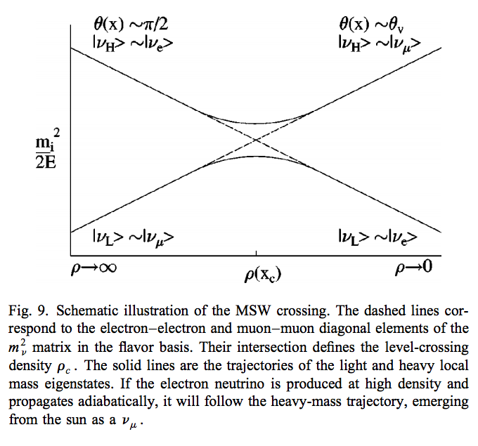
../_images/msw.png — Fig. 5.1 Neutrino physics by Wick C. Haxton and Barry R. Holstein.¶

5.1.2. Solar Neutrinos and MSW Effect¶

The MSW effect itself can be made clear using the example of neutrino oscillations in our sun. In fact it is responsible for the missing solar neutrino problem.

Small Mixing Angle Limit

Just for fun.

Take two flavour mixing as an example.

\[\begin{split}\begin{pmatrix}\nu_e \\ \nu_x\end{pmatrix} = \begin{pmatrix} \cos\theta & \sin\theta \\ -\sin\theta & \cos\theta \end{pmatrix} \begin{pmatrix}\nu_1 \\ \nu_2\end{pmatrix}\end{split}\]

In the small mixing angle limit,

\[\begin{split}\begin{pmatrix}\nu_e \\ \nu_x\end{pmatrix} \to \begin{pmatrix} 1 & \theta \\ -\theta & 1 \end{pmatrix} \begin{pmatrix}\nu_1 \\ \nu_2\end{pmatrix}\end{split}\]

which is very close to an identity matrix. This implies that electron neutrino is more like mass eigenstate \(\nu_1\). By \(\nu_1\) we mean the state with energy \(\frac{ \Delta m^2 }{4E}\) in vacuum.

We need this intuitive picture to understand MSW effect. Electron neutrinos are almost identical to the low mass neutrino mass eigenstate. However, as we will see, due to the matter interaction, the electron flavour neutrino is corresponding to the HEAVY mass eigenstate. This is the key idea in physics of MSW effect.

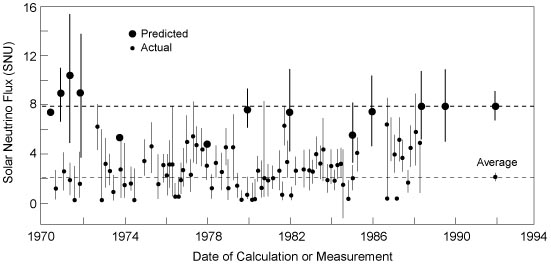
../_images/clorine-detector-solar-neutrinos.jpg — Fig. 5.2 Solar neutrino problem: chlorine detector (Homestake experiment) results and theory predictions. SNU: 1 event for \(10^{36}\) target atoms per second. Source: Kenneth R. Lang (2010)¶

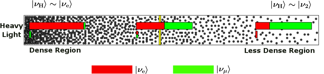
../_images/msw-and-density.png — Fig. 5.3 MSW effect of solar neutrinos. This figure is adapted from Smirnov 2003.¶

Hamiltonian with matter effect is

\[\mathbf{H} = \frac{\lambda(x) - \omega_{\mathrm v} \cos 2\theta_{\mathrm v}}{2} \boldsymbol{\sigma_3} + \frac{ \omega_{\mathrm v} \sin 2\theta_{\mathrm v}}{2} \boldsymbol{\sigma_1}\]

and new basis is defined

\[\begin{split}\begin{pmatrix} \ket{\nu_{\mathrm{e}}} \\ \ket{\nu_{\mu}} \end{pmatrix} = \begin{pmatrix} \cos\theta_{\mathrm m} & \sin\theta_{\mathrm m} \\ -\sin\theta_{\mathrm m} & \cos\theta_{\mathrm m} \end{pmatrix}\begin{pmatrix} \ket{\nu_{\mathrm{L}}} \\ \ket{\nu_{\mathrm{H}}}. \end{pmatrix}\end{split}\]

Now we have two states in this matter basis, the heavy state and the light state. When we talk about adabatic propagation, we mean the system doesn’t jump between these heave and light states.

In the figure, we have dense matter on the left while the matter desnity approaching vacuum on the right. Upper bar means the probability of finding the system to be in heavy state and the lower bar means in light state. As the matter profile doesn’t change too fast, the system undergoes adiabatic propagation and the length of the bars doesn’t change. For example, if the system starts with completely heavy state , it will always remain on heavy state.

Since almost all neutrinos produced in the sun are electron neutrinos, and electron flavor neutrinos experience a big potential, electron flavor almost means heavy state. So we have the system starts with a state that is mostly heavy state and it remains this way. However, during the propagation, heavy state is going to have less electron flavor until some point, we have equal mixing which is MSW resonance. As it approaches vacuum, we have only about 1/3 of the probability to find the neutrinos to be on electron flavor state.

If we discuss more about this phenomenon, we have situations such as not so large density.

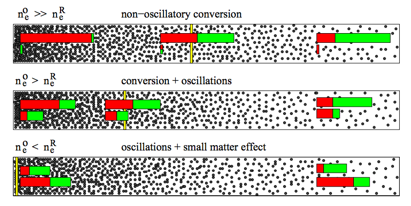
../_images/msw_and_density1.png — Fig. 5.4 MSW conversion for different matter profiles. Smirnov 2003.¶

5.1.3. Visualizing the Solar Neutrino Flavor Oscillations¶

Applying the flavor isospin method (Neutrino Flavour Isospin), we can visualize the flavor conversions.

../_images/matter-effect-large-density.png

../_images/matter-effect-adiabatic-3.png

5.1.4. Numerical Results¶

5.1.4.1. 2 Flavor Oscillation¶

The equation of motion in flavor basis is

\[i\partial_x \Psi_{mf}(x) = \mathbf{H_{mf}} \Psi_{mf}(x)\]

where

\[\mathbf{H_{mf}} = \left( \frac{\Delta}{2} - \frac{\omega}{2} \cos 2\theta_v \right) \boldsymbol{\sigma_3} + \frac{\omega}{2} \sin 2\theta_v \boldsymbol{\sigma_1}.\]

Writing down the dimensionless equation, we have

\[i \partial_{\hat x} \Psi_{mf} = \frac{R_S \omega}{2} ( (\hat\Delta - \cos 2\theta_v ) \boldsymbol{\sigma_3} + \sin 2\theta_v \boldsymbol{\sigma_1} ) \Psi_{mf} .\]

As for the data of the sun I use a simple exponential distribution. The data is also from the paper by Bahcall. The model using just exponential is not accurate however it is enough to make the point in MSW resonance. So I choose a solar model in which the core density is \(n(0) = 10^{-13}\mathrm{GeV}^{3}\). The distribution is

\[n = 10^{-13 - 4.3\hat x} \mathrm{GeV}^{3}.\]

The numerical results can be obtains by plugging this density profile into the differential equation solver.

../_images/numericalMSW-model-3.png — Fig. 5.5 Numerical results for electron flavor neutrino probability and the other flavor neutrino probability when the electron density profile is \(10^{-14 - 4.3\hat x} \mathrm{GeV}^{3}\).¶

../_images/numericalMSW-model-2flavor-minus13-1.png — Fig. 5.6 Number density profile \(n(\hat x) = 10^{-13 - 4.3\hat x}\mathrm{GeV^{3}}\).¶

Since we can easily predict the survival probability using simple theory. Here are some comparision. The following figures are for matter profile \(10^{-13-4.3\hat x}\mathrm{GeV^3}\) and vacuum oscillation frequency \(\omega = 10^{-20} \mathrm{GeV}, 10^{-19} \mathrm{GeV},10^{-18} \mathrm{GeV},10^{-17} \mathrm{GeV}\) respectively. As we can see that in this two flavor special case, the problem doesn’t dependent on energy and mass difference independently but depends only on \(\omega=\frac{\Delta m^2}{2E}\). If we choose \(\Delta m^2=7.5\times 10^{-5}\mathrm{eV^2}\), the four figures are corresponding to energies \(7.5\mathrm{MeV},0.75\mathrm{MeV},7.5\times 10^{-2}\mathrm{MeV},7.5\times 10^{-3}\mathrm{MeV}\).

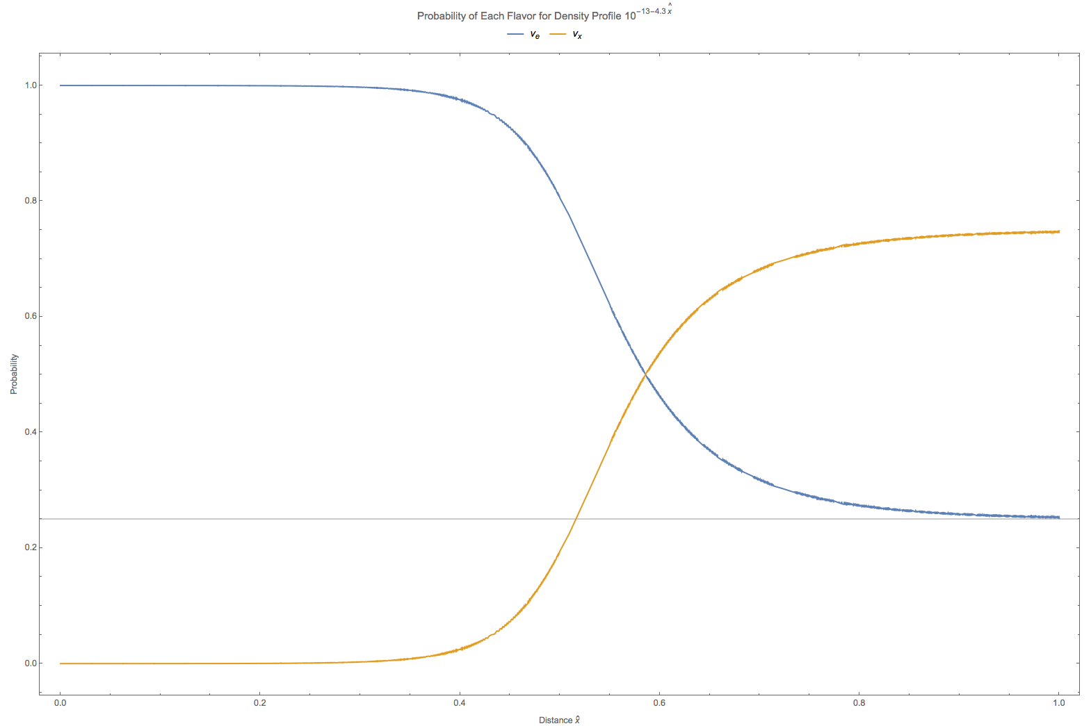
../_images/compThNu13-1.png — Fig. 5.7 The grey line is theoretical survival probability at \(\hat x = 1\). In this calculation the vacuum oscillation frequency is set to \(\omega = 10^{-20} \mathrm{GeV}\).¶

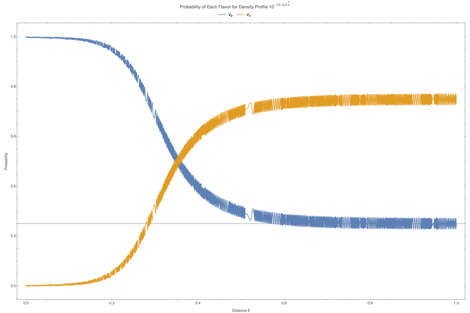
../_images/compThNu13-2.png — Fig. 5.8 The grey line is theoretical survival probability at \(\hat x = 1\). In this calculation the vacuum oscillation frequency is set to \(\omega = 10^{-19} \mathrm{GeV}\).¶

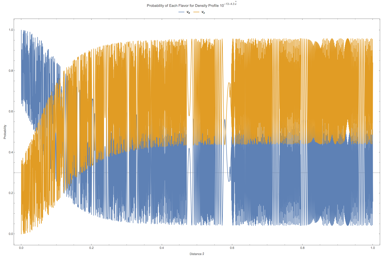
../_images/compThNu13-3.png — Fig. 5.9 The grey line is theoretical survival probability at \(\hat x = 1\). In this calculation the vacuum oscillation frequency is set to \(\omega = 10^{-18} \mathrm{GeV}\).¶

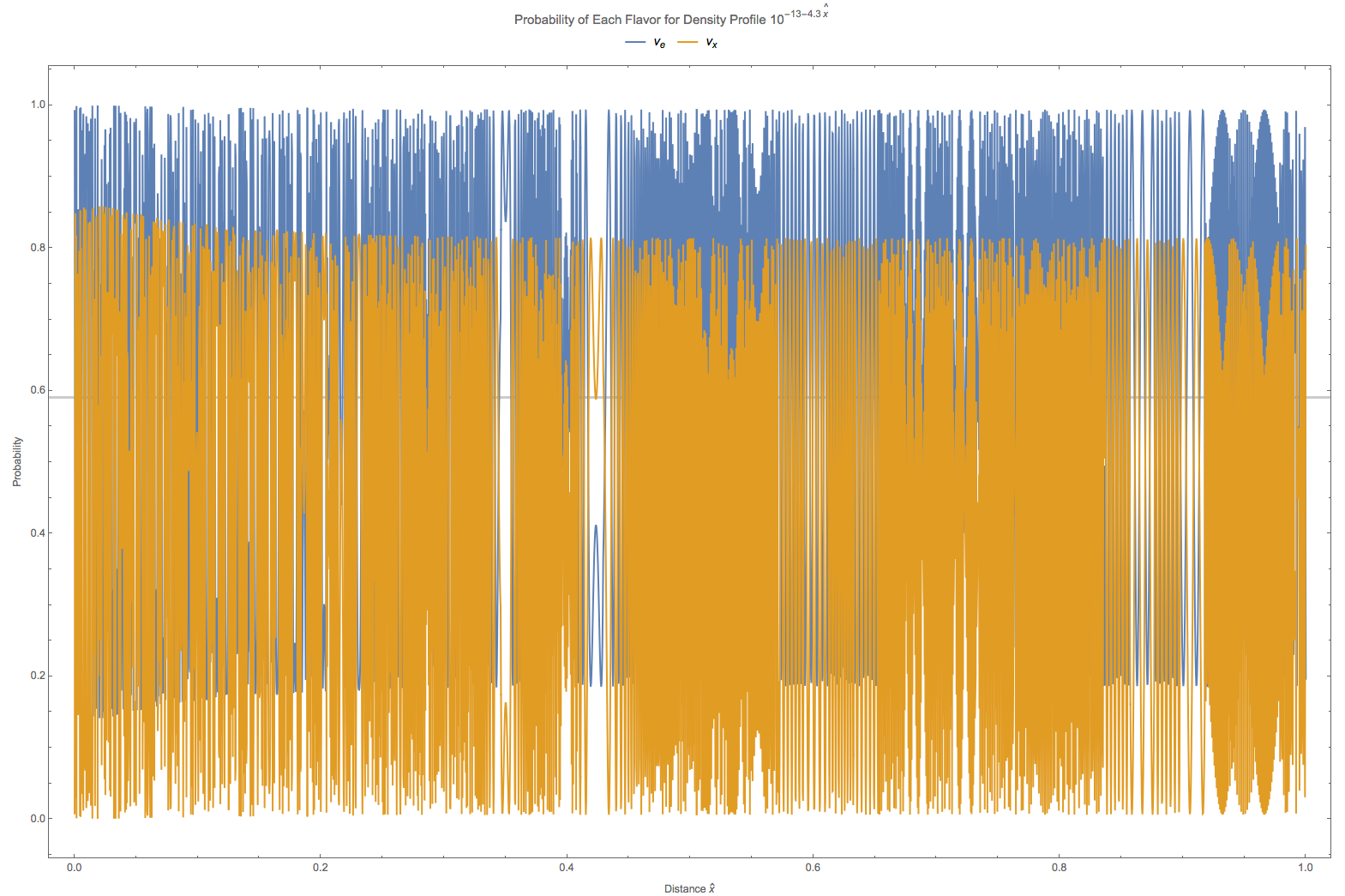
../_images/compThNu13-4.png — Fig. 5.10 The grey line is theoretical survival probability at \(\hat x = 1\). In this calculation the vacuum oscillation frequency is set to \(\omega = 10^{-17} \mathrm{GeV}\).¶

5.1.4.2. Three flavor Oscillations¶

Vacuum part of the Hamiltonian is

\[\begin{split}\mathbf{H_{mvv}} = \frac{1}{2E} \begin{pmatrix} m_1^2 & 0 & 0 \\ 0 & m_2^2 & 0 \\ 0 & 0 & m_3^2 \end{pmatrix}.\end{split}\]

The matter interaction in flavor basis is

\[\mathbf{V_{mf}} = \sqrt{2}G_F n \mathrm{diag}{1,0,0}.\]

Thus to work in vacuum mass eigenstates, we need a transformation

\[\mathbf{V_{mv}} = \mathbf{U^{-1}}\mathbf{V_{mf}} \mathbf{U}.\]

Then the Hamiltonian becomes

\[\begin{split}\mathbf{H_{m}} = \begin{pmatrix} \frac{m_1^2}{2E} + \Delta U_{e1}^2 & \Delta U_{e1} U_{e2} & \Delta U_{e1} U_{e3} \\ \Delta U_{e2} U_{e1} & \frac{m_2^2}{2E} + \Delta U_{e2}^2 & \Delta U_{e2} U_{e3} \\ \Delta U_{e3} U_{e1} & \Delta U_{e3} U_{e2} & \frac{m_3^2}{2E} + \Delta U_{e3}^2 \end{pmatrix}\end{split}\]

Trace of this Hamiltonian is \(\mathrm{Tr}(\mathbf{H_m}) = \frac{m_1^2+m_2^2+m_3^2}{2E}+\Delta\). To find the traceless part, we can use the relation [ohlsson2000]

\[M = M_{traceless}+ \frac{1}{N} \mathrm{Tr}(M) I,\]

where \(N\) is the rank.

The traceless part of Hamiltonian becomes

\[\begin{split}\mathbf{H_{m}} = \begin{pmatrix} \Delta U_{e1}^2 - \frac{1}{3}\Delta + \frac{1}{3}(\frac{m_1^2-m_2^2 + m_1^2-m_3^2}{2E}) & \Delta U_{e1}U_{e2} & \Delta U_{e1} U_{e3} \\ \Delta U_{e2} U_{e1} & \Delta U_{e2}^2 -\frac{1}{3}\Delta + \frac{1}{3}\frac{m_2^2 - m_1^2+m_2^2-m_3^2}{2E} & \Delta U_{e2}U_{e3} \\ \Delta U_{e1} U_{e3} & \Delta U_{e2} U_{e3} & \Delta U_{e3}^2 -\frac{1}{3} \Delta + \frac{1}{3} \frac{m_3^2 - m_1^2 + m_3^2-m_2^2 }{2E} \end{pmatrix}.\end{split}\]

Define the following quantities where only two of them are linearly independent

\[\begin{split}\Delta m_{12}^2 & = m_2^2 - m_1^2 \\ \Delta m_{23}^2 & = m_3^2 - m_2^2 \\ \Delta m_{13}^2 & = m_3^2 - m_1^2.\end{split}\]

We define an energy scale related to the radius of the sun

\[\epsilon_S = \frac{1}{R_S}.\]

The EoM can be written in a dimensionless manner,

\[\begin{split}i\partial_{\hat x} \Psi_{m} = \begin{pmatrix} \tilde\Delta U_{e1}^2 - \frac{1}{3}\tilde\Delta + \frac{1}{3}(\frac{\Delta m_{12}^2 + \Delta m_{13}^2}{2E\epsilon_S}) & \tilde\Delta U_{e1}U_{e2} & \tilde\Delta U_{e1} U_{e3} \\ \tilde\Delta U_{e2} U_{e1} & \tilde\Delta U_{e2}^2 -\frac{1}{3}\tilde\Delta + \frac{1}{3}\frac{\Delta m_{12}^2 + \Delta m_{23}^2}{2E\epsilon_S} & \tilde\Delta U_{e2}U_{e3} \\ \tilde\Delta U_{e1} U_{e3} & \tilde\Delta U_{e2} U_{e3} & \tilde\Delta U_{e3}^2 -\frac{1}{3} \tilde\Delta + \frac{1}{3} \frac{\Delta m_{13}^2 + \Delta m_{23}^2 }{2E\epsilon_S} \end{pmatrix}\Psi_m ,\end{split}\]

where \(\tilde\Delta = \Delta/\epsilon_S\).

The parameters for this calculation in units of \(GeV^{\mathrm{some power}}\) are

\[\begin{split}n(x) &= 10^{-12 - 4.3 x} \\ \epsilon_S &= 10^{-24}\\ \tilde\Delta(x) &= \sqrt{2} G_F n(x)/\epsilon_S\\ \Delta m _ {12}^2 &= 7.6\times 10^{-5}\times 10^{-18}\\ \Delta m _ {13}^2 &= 2.3\times 10^{-3}\times 10^{-18}\\ \Delta m _ {23}^2 &= \Delta m _ {13}^2 - \Delta m _ {12}^2\\ E &= 10^{-3}\end{split}\]

For these parameters there is only resonance for \(\Delta m_{13}^2+\Delta m_{23}^2\).

A quick check over the different energy scales.

Vacuum energy scales in normal hierarchy

\[\begin{split}\omega_{12}&= \frac{\Delta m_{12}^2}{2E} = 3.8\times 10^{-20}\mathrm{GeV}\\ \omega_{13}&= \frac{\Delta m_{13}^2}{2E} = 1.7\times 10^{-18}\mathrm{GeV}\\ \omega_{23}&= \frac{\Delta m_{23}^2}{2E} \approx \omega_{13}\end{split}\]
Matter related scale for density profile \(10^{-14-4.3\hat x}\)

\[\Delta_1 = 1.6\times 10^{-19-4.3\hat x}\in [1.6\times 10^{-23.3},1.6\times 10^{-19}]\]
Matter related scale for density profile \(10^{-13-4.3\hat x}\)

\[\Delta_1 = 1.6\times 10^{-18-4.3\hat x}\in [1.6\times 10^{-22.3},1.6\times 10^{-18}]\]

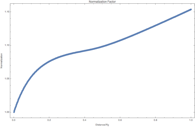
../_images/numericalMSW3Flavor-normalization.png — Fig. 5.11 Normalization factor as a function of distance.¶

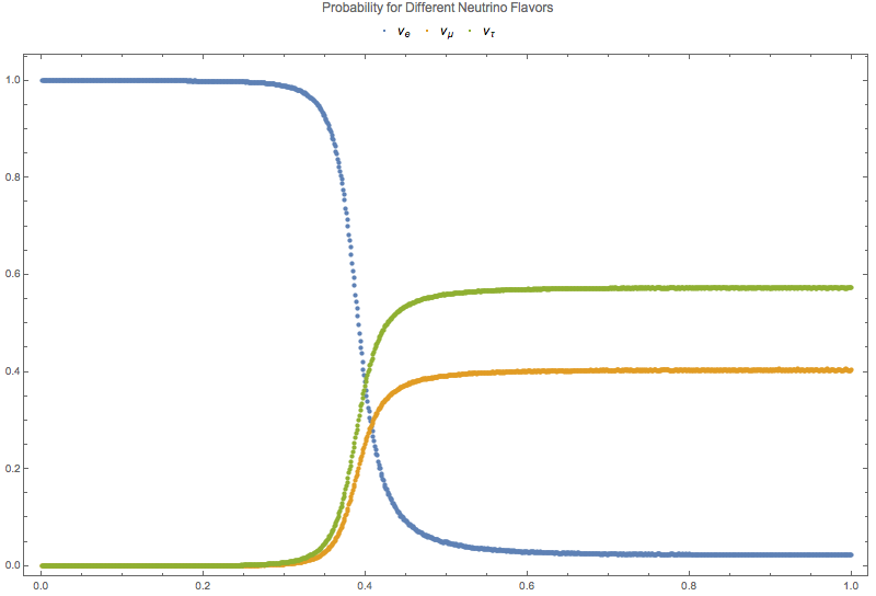
../_images/numericalMSW3Flavor-probabilities.png — Fig. 5.12 Probability for each flavor of neutrinos.¶

Applying a number density function \(n(x) = 10^{-13 - 4.3 x}\) to the system, the small scale oscillations are revived,

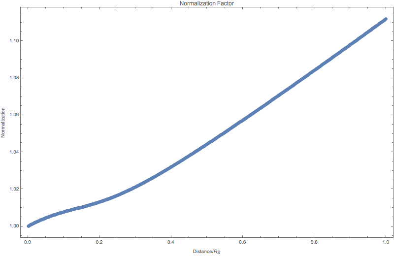
../_images/numericalMSW3Flavor-2-norm.png — Fig. 5.13 Normalization of the states for numerical 3 flavor oscillation in the sun with density profile \(10^{-13 - 4.3 x}\).¶

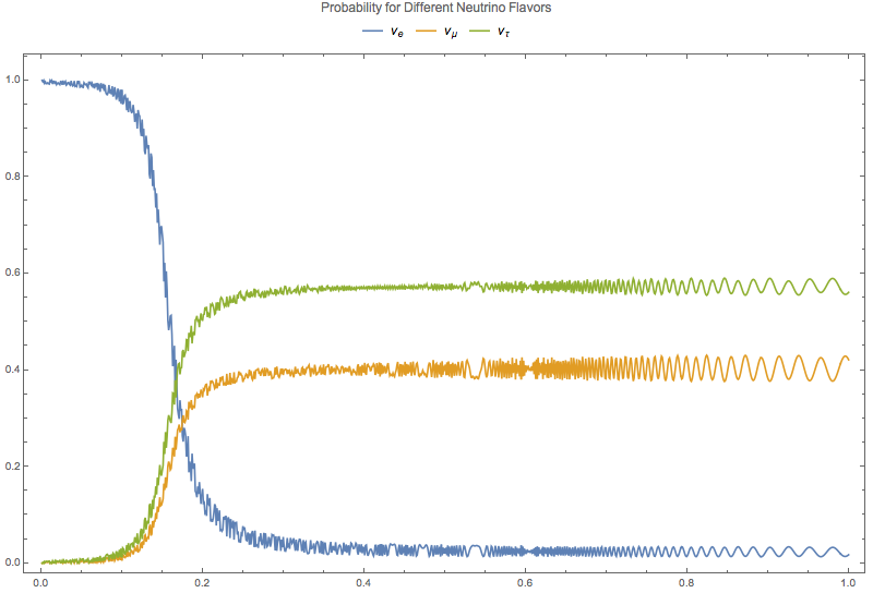
../_images/numericalMSW3Flavor-2-probability.png — Fig. 5.14 Numerical results for 3 flavor oscillation in the sun with density profile \(10^{-13 - 4.3 x}\).¶

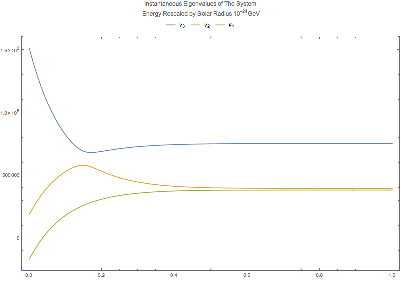
../_images/numericalMSW3Flavor-minus13-Inst-Eigen-Energies.png — Fig. 5.15 Eigenenergies for density profile \(10^{-13 - 4.3 x}\).¶

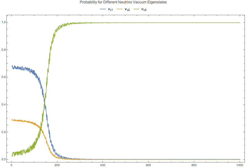
../_images/numericalMSW3Flavor-vac-eigen-prob.png — Fig. 5.16 Survival probabilities for different vacuum mass eigenstates for 3 flavor oscillation in the sun with density profile \(10^{-13 - 4.3 x}\).¶

An interesting notion is the survival probability for the instantaneous eigenstates.

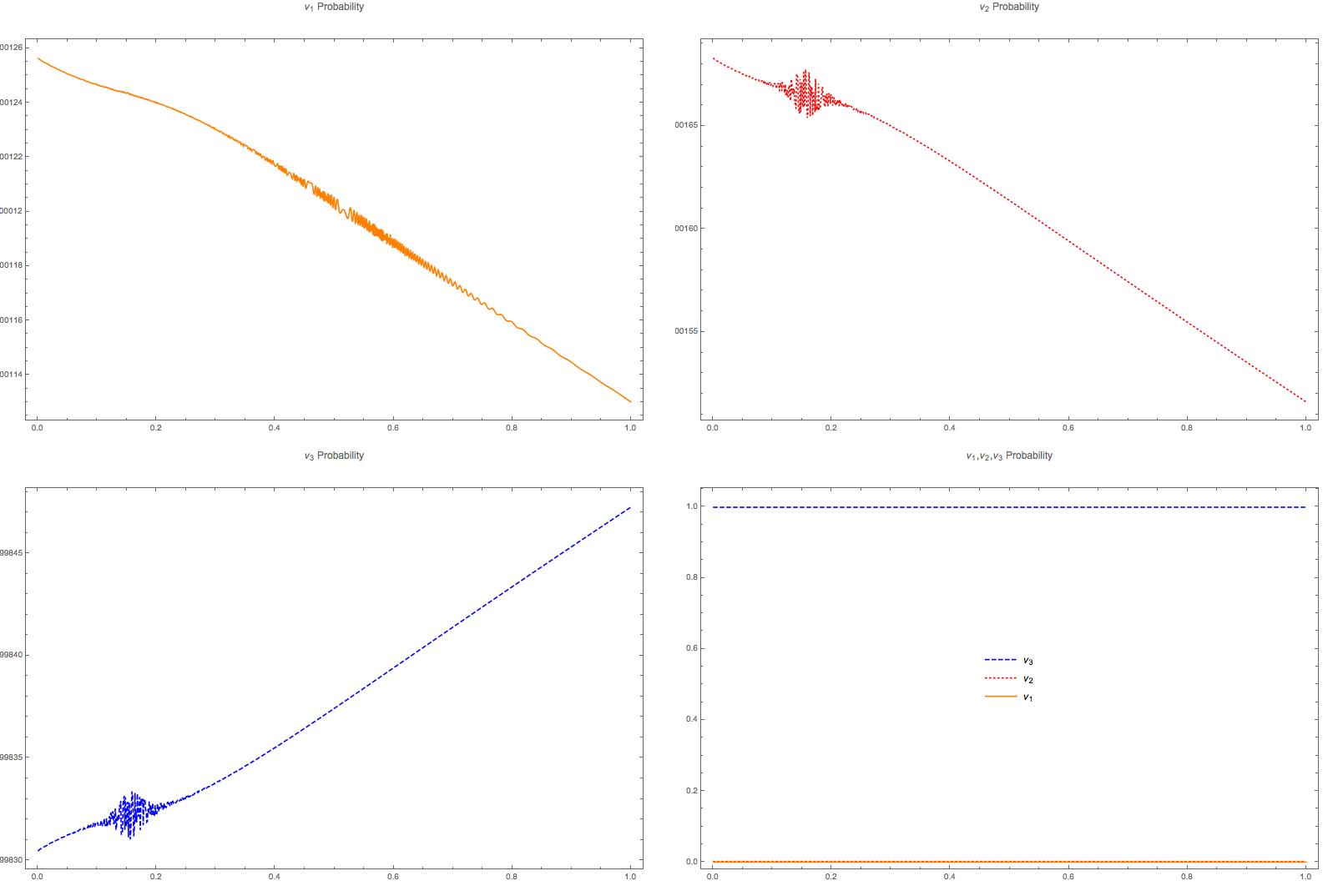
../_images/instanEigenstetes-minus13-Grid.png — Fig. 5.17 Probability for the instantaneous eigenstates for matter profile \(10^{-13 - 4.3 x}\).¶

Lower matter density will have less suppression on vacuum oscillations.

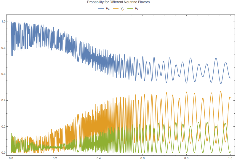
../_images/numericalMSW3Flavor-minus14matter.png — Fig. 5.18 Numerical results for 3 flavor oscillation in the sun with density profile \(10^{-14 - 4.3 x}\).¶

ohlsson2000: Ohlsson, T., & Snellman, H. (1999). Three flavor neutrino oscillations in matter, 2768(2000), 25. doi:10.1063/1.533270

5.1.4.3. Ternary Diagram¶

High matter density suppresses the vacuum oscillations which is clearly shown on a ternary diagram.

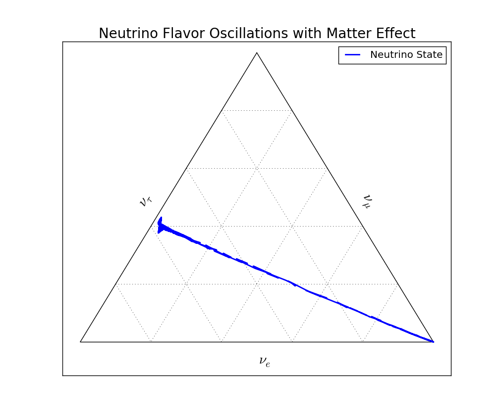
../_images/mass-1.png — Fig. 5.19 Ternary diagram for MSW effect shows that the vacuum oscillations in this case is suppressed. Comparing this with the survival probability, the survival probability for electron neutrino drops to a value and the rapid oscillations start to show up. The drop is the movement in the ternary diagram from the right-bottom cornor to the tau neutrino axis. These rapid oscillations corresponds to the T-shaped tip at the other end of the line.¶

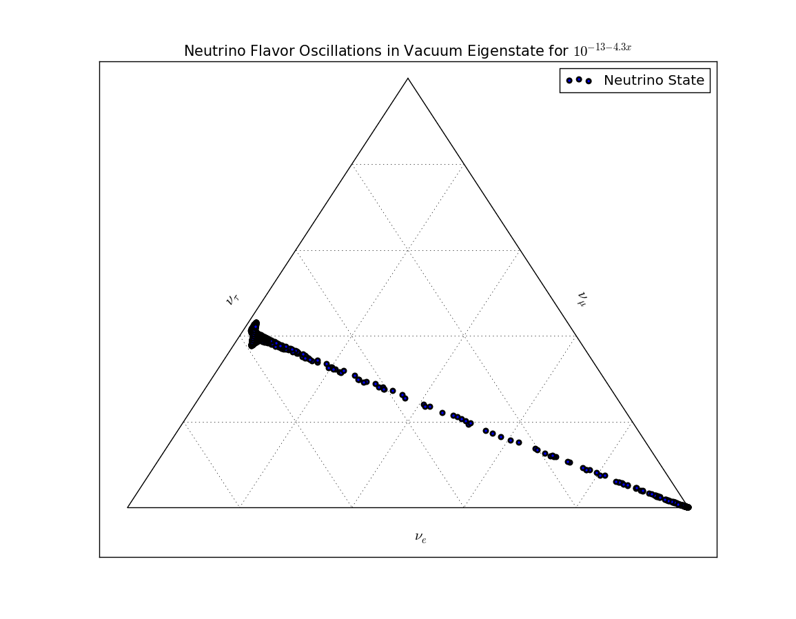
../_images/mass-1-scatter.png — Fig. 5.20 Ternary diagram for MSW effect with homogeneously descretized position \(x\) with matter profile \(10^{-13-4.3x}\mathrm{GeV^3}\). We can see clearly that the system stays on the two ends to the line for a longer time that in the middle where the transition happens very quickly. This can also be seen in the survival probability plot.¶

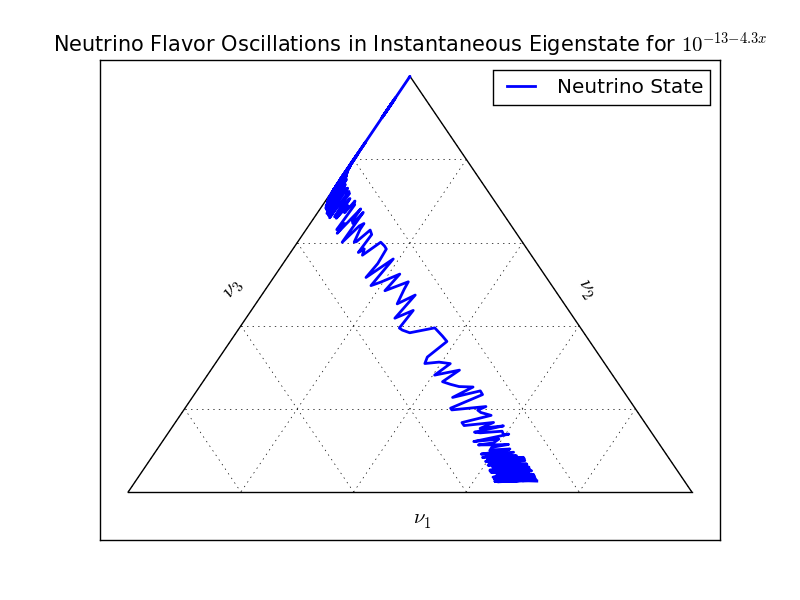
../_images/matter-inst-eigen-e-1.png — Fig. 5.21 Ternary diagram for instantaneous eigenstates with matter profile \(10^{-13-4.3x}\mathrm{GeV^3}\). The system starts from almost the second instantaneous state then moves along the state that \(\nu_1=0\).¶

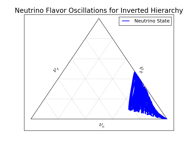
../_images/matter-inverted-1.png — Fig. 5.22 Ternary diagram for MSW effect with inverted hierarchy \(\Delta m_{23} = m_3^2 - m_2^2<0\). The shape changes a lot since the frequencies changes a lot.¶

5.1.5. Experiments¶

MSW effect is verified by serveral experiments, SNO, Borexino and many others.

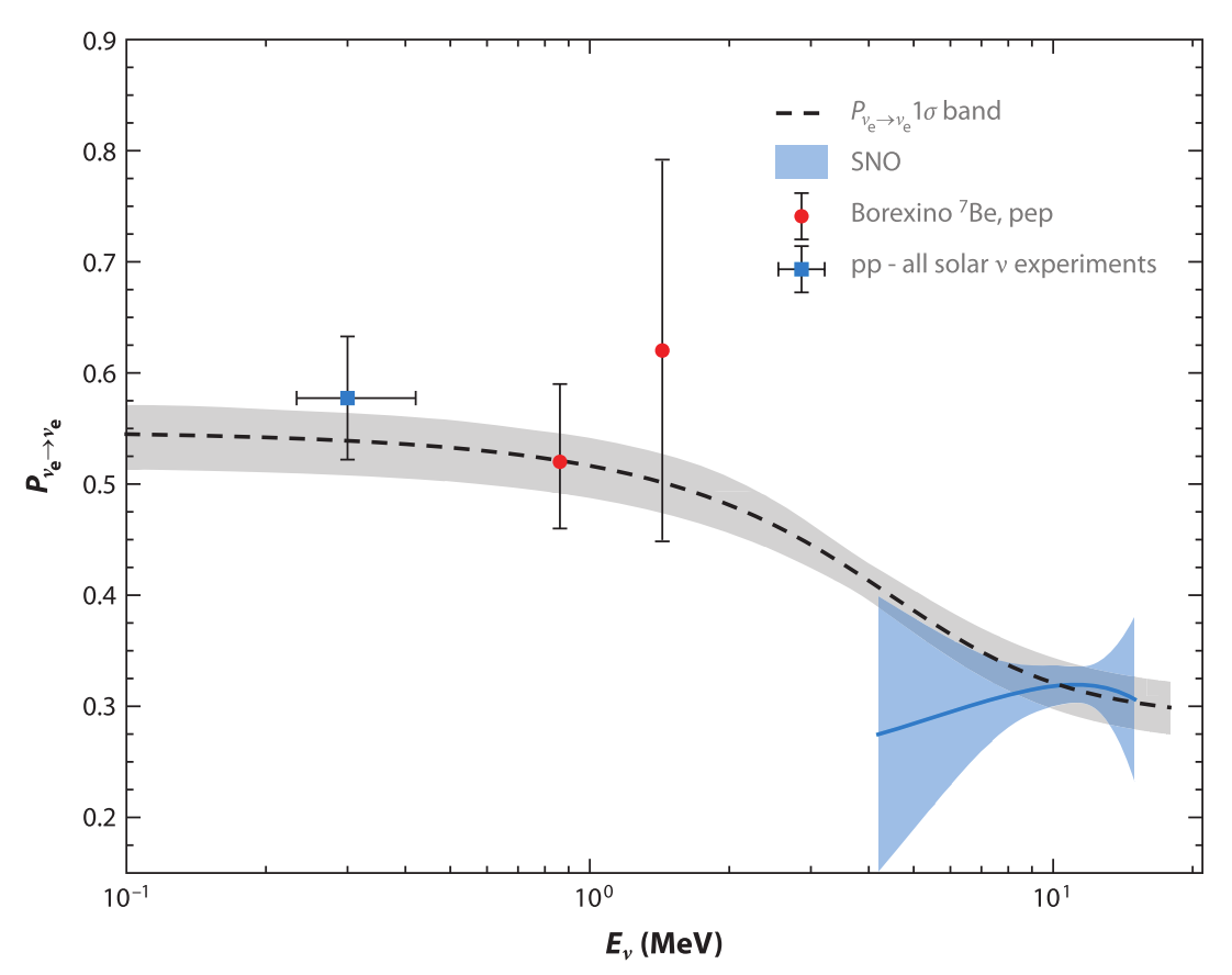
../_images/msw-experiments.png — Fig. 5.23 Comparison of MSW prediction and experiments. The uncertainties of MSW prediction line are on on mixing angles. Figure from Haxton et al 2013.¶

5.1.6. MSW Triangle¶

Finally, one of the interesting things about MSW effect is that we could find a triangle where the survival probability is low.

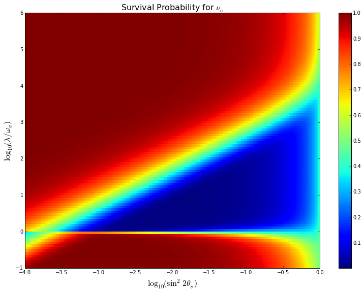
../_images/msw-triangle.png — Fig. 5.24 Code and illustration for the calculation can be downloaded on github https://github.com/NeuPhysics/codebase/blob/master/ipynb/matter/msw_triangle.ipynb .¶

5.1.7. Refs and Notes¶

Wolfenstein, L. (1978). Neutrino oscillations in matter. Physical Review D, 17(9), 2369–2374. doi:10.1103/PhysRevD.17.2369
Wolfenstein, L. (1979). Neutrino oscillations and stellar collapse. Physical Review D, 20(10), 2634–2635. doi:10.1103/PhysRevD.20.2634
Parke, S. J. (1986). Nonadiabatic Level Crossing in Resonant Neutrino Oscillations. Physical Review Letters, 57(10), 1275–1278. doi:10.1103/PhysRevLett.57.1275
Bethe, H. A. (1986). Possible Explanation of the Solar-Neutrino Puzzle. Physical Review Letters, 56(12), 1305–1308. doi:10.1103/PhysRevLett.56.1305