3.2. Concepts in Experiments
Chapter 7 (section 7.6) and chapter 12 of Giunti’s book 1 are the good materials to read.
3.2.1. Prediction of Theory
In experiments we do not directly measure the exact survival probabilty, instead we measure events that are generated by neutrinos. The connection between the theoretical exact survival probability is to average over the parameters that we do not precisely resolve.
In the example of 2 flavor oscillation, the transition probability from \(\nu_\alpha\) to \(\nu_\beta\) is given by
It is not possible to obtain this result since we do not have enough resolution for \(L\) and \(E\). The observed result is the probability averaged over the distribution of \(L\) and \(E\). 1
Nonetheless, in this simple two flavor example, the probability only depends on \(\frac{L}{E}\). So we average over \(\frac{L}{E}\). 1
where \(\phi(L/E)\) is the distribution.
The practical distribution of \(\frac{L}{E}\) is Gaussian, 1
which determines the average of the cosine term is 1
Variance of L/E
The virance can be splitted into two parts,
which comes from the fact that a Gaussion is written as
3.2.1.1. What Does A Detector Do
In experiments we can either detect the appearance of \(\nu_\alpha\) or find the disappearance of \(\nu_\alpha\) given a source of \(\nu_\beta\).
If a detector can not observe any oscillations, that means it can only put a upper limit on the averaged probability. Otherwise the detector will find exactly the averaged probability!
That being said, the averaged probability obtains an upper limit through experiments,
which in 2 flavor case is
Using Gaussian distribution of \(\phi(L/E)\), we have 1
The relation between \(\sin^2 2\theta_v\) and \(L/E\) can be found,
in a simple equation,
This relation allows us to do a joint analysis of \(\sin^2 2\theta_v\) and \(\Delta m^2\).
General Form of Constraint
Rewrite
we have
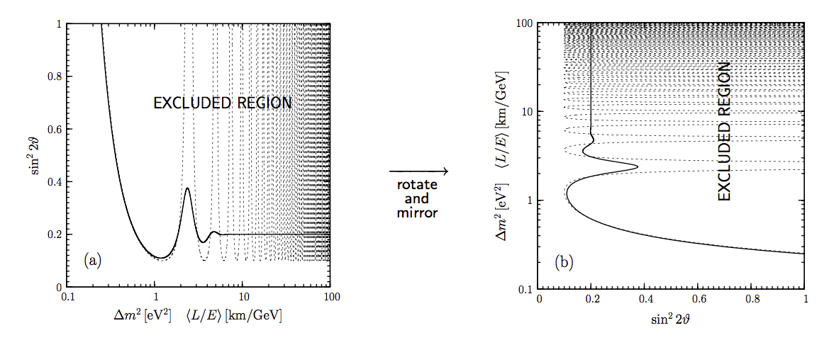
Fig. 3.2 A figure grabbed from Giunti’s book Fundamentals of Neutrino Physics and Astrophysics section 7.6. As we mentioned, we have a relation between \(\sin^2 2\theta_v\) and \(\Delta m^2\), which is given as the black solid lines in the figures. The regions that have larger values of \(\sin ^2 2\theta_v\) are excluded. Thus the solid lines are called exclusion curve.
3.2.1.2. The Stringent Constraint of Mixing Angle
The most stringent constraint for \(\sin^2 2\theta_v\) happens when the demoninator of the right side is largest, which means
Averge of cosine
In experiments, we have the fact that the change in \(\frac{L}{E}\) is small compared to the average value \(\langle\frac{L}{E}\rangle\).
So when we average over the cosine
we actually can assume that we are averaging over the argument. The reason is that we can do Taylor expansion and drop all terms except the zeroth order since the change in argument is small.
In the language of math,
The left hand side can be expanded to
which is pluged into the inequality. We have finally
The condition leads to
Solving this equation we know the condition for the most stringent constraint on \(\sin^2 2\theta_v\) happens when
which is
Units of \(\Delta m^2 L/E\)
First of all, calculate the following expression,
Thus we have
Rewrite it using the Bethe trandition,
3.2.1.3. Small \(\Delta m^2 \langle L/E \rangle\) Limit
In small \(\Delta m^2 \langle L/E \rangle\) limit, we have the Taylor expansion of cosine term
Using the Gaussian distribution result, we reach a constraint
As we have discussed before,
which leads to
Giunti’s Results
Giuti’s idea is that
basically means
which leads to the result that
Then he has
3.2.1.4. Large \(\Delta m^2 \langle L/E \rangle\) Limit
In this limit, we have a flat line in the \(\sin^2 2\theta_v\) vs \(\Delta m^2 \langle\frac{L}{E}\rangle\) plot.
The reason is that the limit of \(\sin^2 2\theta_v\) becomes
Reason for Flat Line
The exponential part dominates and the denominator becomes 1 at large \(\Delta m^2 \langle L/E \rangle\) value.
3.2.2. Sensitivity
Sensitivity
\((\sin^2 2\theta_v)_s\) and \((\Delta m^2)_s\) are better at small values because they means the “smallest” constraint we can obtain.
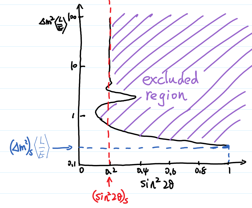
Fig. 3.3 Sensitivities
For disappearance experiments:
L \(\searrow\) : \((\sin^2 2\theta_v)_s\) \(\searrow\), \((\Delta m^2)_s\) \(\nearrow\); (going up means sensitivity becomes worse; going down means sensitivity becomes better.)
E \(\searrow\) : \((\sin^2 2\theta_v)_s\) \(\searrow\), \((\Delta m^2)_s\) \(\searrow\).
We have very little control over the production energy of neutrinos though. To have a better sensitivity of mass difference (i.e., make the sensitivity values smaller), we need to have a bigger distance, which makes the sensitivity of mixing angles worse. But we can at the same time increase the flux of \(\nu_\alpha\) and the mass of the detector to compensate this loss of sensitivity.
3.2.3. Review of Experiments
Through the analysis we know that the most important factors of experiments are
Basiline \(L\);
Source neutrino flux;
Neutrino energy \(E\).
3.2.3.1. Reactor Experiments
What we would like to see in the experiments is the disappearance of the reactor neutrinos. In nuclear fusion we have a lot of \(\bar\nu_e\) which will oscillate to other flavors. If the detector is sensitive enough we would find out that the detected neutrinos are smaller than the expected neutrinos without oscillation.
The energy of the neutrinos is about 1.8MeV.
The first question is how many neutrinos can be detected. If neutrino energy is too high, cross section at detector will be large but neutrino flux per unit energy will be small. The best detection rate is at some certain energy.
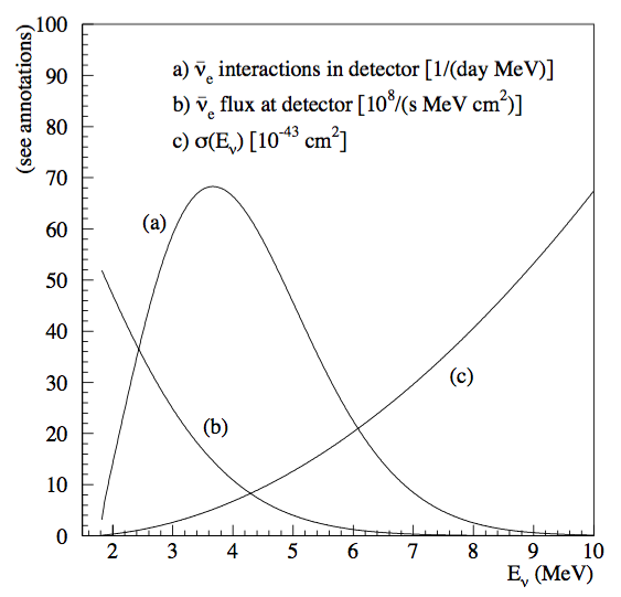
Fig. 3.4 The best energy of detection. Figure 12.2 in Giunti’s book.
The Source Flux
We can calculate the production of neutrinos by monitoring the power of the nuclear reactor.
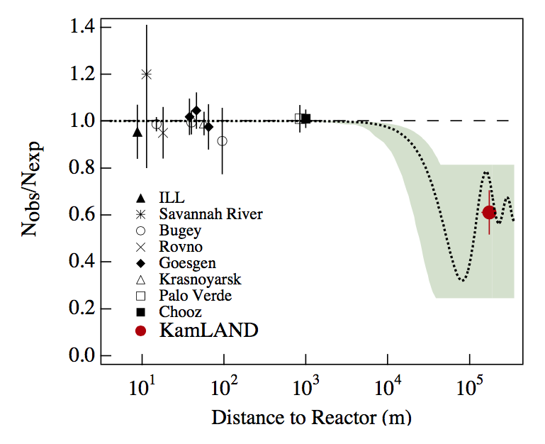
Fig. 3.5 The ratio of observed neutrino flux to expected neutrino flux compared in different experiments. The dotted line is the ratio when expected flux calculated from best fit results of \(\Delta m^2\) and \(\sin^2 2\theta_v\) extracted from solar neutrino experiments. These experiments more or less lie on the best fit result. Figure 12.3 of Giunti’s book.
\(L\sim 10 - 100 m\) : short baseline experiment (SBL);
CHOOZ and Palo Verde has baseline \(L\sim 1km\) : long baseline experiment (LBL);
KamLAND has baseline \(L\sim 200km\) : Very long baseline experiment (VLBL).
To find the best result of mass squared difference \(\Delta m^2\), we need a long baseline like KamLAND.
Background
One of the background of neutrinos is the cosmic ray. The cosmic neutrino background is much smaller than the reactor neutrino flux.
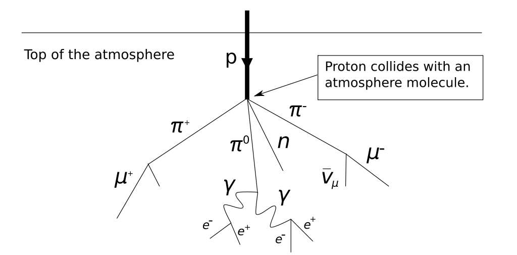
Fig. 3.6 Production of neutrinos through cosmic rays. We need to shield the hardons. From wikipedia.
The background actually can be measured when the nuclear plants are turned off to supply fuel.
3.2.3.1.1. Review of Reactor Experiments
Experiments can detect antielectron neutrinos through inverse neutron decay (inverse beta decay),
Late 1970s to the 1990s, SBL experiments with detector mass of order \(10^2\mathrm{kg}\) got null results, i.e., they didn’t find the disappearance of the reactor neutrinos which is \(\bar\nu_e\). The reason is that they have short baseline. The result is \(\Delta m^2\sim 10^{-2}\mathrm{eV^2}\).
LBL experiments gave us better exclusion curves. * CHOOZ : 5 tons of detector mass; 1115km and 998m from the two sources. * Palo Verde : 12 tons of detector mass; 890m, 890m and 750m from the three sources.
KamLAND: mostly detects neutrinos from 53 reactors in Japan. 80% neutrinos from reactors at distance between 140km and 215km. 3000 tons of detector mass. Best fit results using KamLAND and solar neutrino is \(\Delta m^2 = 7.9^{+0.6}_{0.5}\times 10^{-5}\mathrm{eV^2}\) and \(\tan^2\theta_v = 0.40^{+0.10}_{-0.07}\), which corresponds to \(\sin^2 2\theta_v \sim 0.82\).
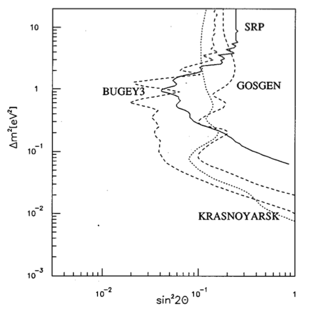
Fig. 3.7 SBL results from Giunti’s book (figure 12.5). These experiments showed exclusion curves that extend to \(\Delta m^2\sim 10^{-2}\mathrm{eV^2}\).
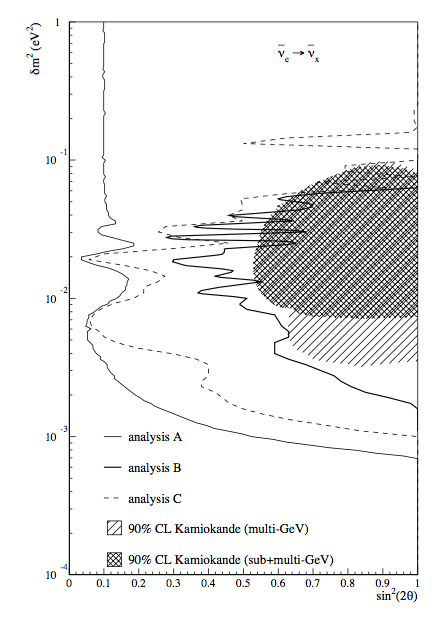
Fig. 3.8 CHOOZ result from Giunt’s book (figure 12.6).
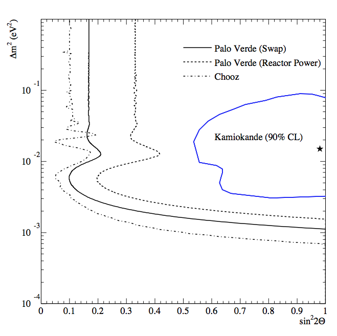
Fig. 3.9 Palo Verde result from Giunt’s book (figure 12.7).
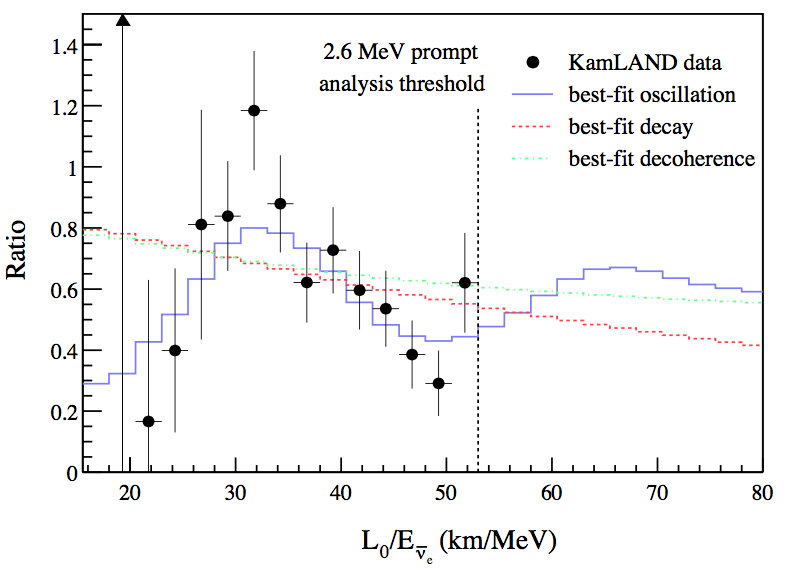
Fig. 3.10 KamLAND detected the oscillation. To calculate the expected flux, the experiment used \(L_0 = 180 \mathrm {km}\). The best fit is \(\Delta m^2 7.9^{+0.6}_{-0.5} times 10^{-5}\mathrm{eV^2}\). From Giunti figure 12.9.
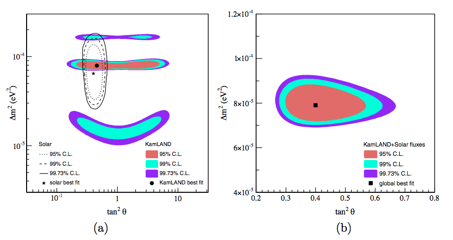
Fig. 3.11 KamLAND result from Giunt’s book (figure 12.10). The left figure is the result of KamLAND while the result is the joint analysis of KamLAND and solar neutrino using 2 neutrino oscillation.
3.2.3.2. Accelerator Experiments
WB : wide band = wide energy spectrum;
NB : narrow band = narrow energy spectrum;
OA : off-axis to obtain almost monochromatic beam.
3.2.4. Low Energy Neutrino Detection
[KATRIN](https://www.katrin.kit.edu/)
Project 8
PROLEMY