1.2.1. Fast Modes¶

1.2.1.1. Why is it fast?¶

Fast modes require different opening angles for neutrinos and anti-neutrinos. The reason seems to be quite understandable. Forward scattering requires “colliding beams”. In the early studies of neutrino self interactions, the models always have same opening angles for neutrinos and antineutrinos, which means that no colliding for neutrinos and antineutrinos on the same side of emission.

Different opening angles for all beams introduce collisions between all the beams, thus possibly leading to more conversions.

Here we use the four beams model. The linear stability analysis is simply four coupled harmonic oscillators.

How could they be harmonic oscillators?

Here is the confusion. How could \(\epsilon\) become very large if they are coupled harmonic oscillators? Is this related the fact that \(\epsilon\) is complex instead of real?

We take out the terms related to the difference in opening angles \(\chi_-=1-\cos(\theta_1 - \theta_2)\). The linearized equation of motion becomes

\[\begin{split}i \partial_z \begin{pmatrix} \epsilon^L \\ \bar\epsilon^L \\ \epsilon^R \\ \bar\epsilon^R \end{pmatrix} = \begin{pmatrix} \frac{ -\mu\alpha \chi_- }{\sin\theta_1} & \frac{ \mu\alpha\chi_- }{\sin\theta_1} & 0 & 0 \\ \frac{ -\mu\chi_- }{\sin\theta_2} & \frac{ \mu\chi_- }{\sin\theta_2} & 0 & 0 \\ 0 & 0 & \frac{ -\mu\alpha\chi_- }{\sin\theta_1} & \frac{ \mu\alpha\chi_- }{\sin\theta_1} \\ 0 & 0 & \frac{ -\mu\chi_- }{\sin\theta_2} & \frac{ \mu\chi_- }{\sin\theta_2} \end{pmatrix} \begin{pmatrix} \epsilon^L \\ \bar\epsilon^L \\ \epsilon^R \\ \bar\epsilon^R \end{pmatrix}.\end{split}\]

The matrix becomes block diagonalized. We assume a solution of the form \(\epsilon = \epsilon_0 e^{i\Omega}\) which is substitued into the equation. The first two components obey the equation.

\[\begin{split}\begin{pmatrix} \mu M_{11} + \Omega & \mu M_{12} \\ \mu M_{21} & \mu M_{22} + \Omega \end{pmatrix} \begin{pmatrix} \epsilon^L \\ \bar \epsilon^L \end{pmatrix} =0.\end{split}\]

The solutions of \(\Omega\) has the form

\[\Omega = \frac{ -(M_{11} + M_{22}) \pm \sqrt{\Delta} }{ 2 } \mu \propto \mu,\]

where the discrimination \(\Delta\) is

\[\Delta = (M_{11} - M_{22})^2 + 4 M_{12} M_{21}.\]

1.2.1.2. Several Numerical Calculations¶

Four Beams Model

There are many things to consider for the four beams line model.

Different emission angle for neutrinos and antineutrinos;
Different density for neutrinos and antineutrinos;
Left and right difference.

Is the system unstable even for \(\omega_v=0\) and \(\lambda=0\)?

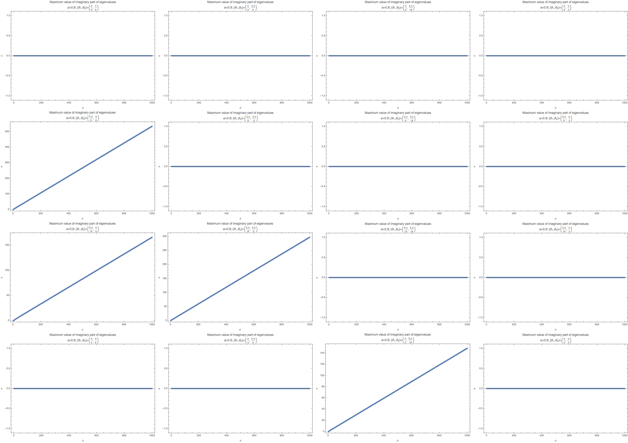
../../_images/fast-mode-alpha-0.8.png — Fig. 1.49 The maximum imaginary part in linear stability analysis. These calculations are for fix \(k_m/\hat E=1\), where \(\hat E\) is the energy scale used to scale all the quantities.¶

\[\begin{split}\omega_v =& 0\\ \lambda =& 0\\ \alpha = & 0.8.\end{split}\]

The grid of figure are arranged according to the following values of \(\{\theta_1,\theta_2\}\).

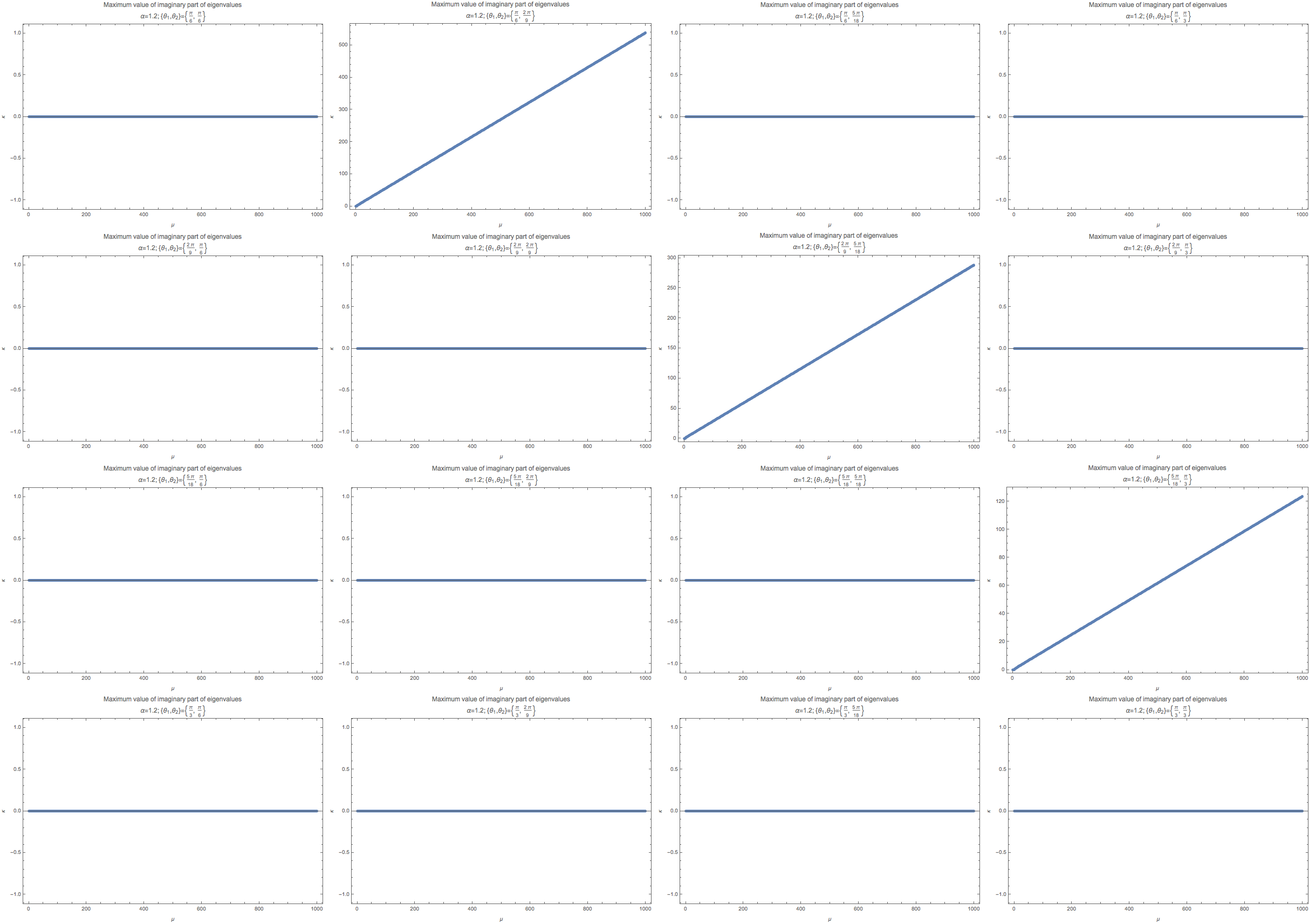
\[\begin{split}\begin{array}{cccc} \left\{\frac{\pi }{6},\frac{\pi }{6}\right\} & \left\{\frac{\pi }{6},\frac{2 \pi }{9}\right\} & \left\{\frac{\pi }{6},\frac{5 \pi }{18}\right\} & \left\{\frac{\pi }{6},\frac{\pi }{3}\right\} \\ \left\{\frac{2 \pi }{9},\frac{\pi }{6}\right\} & \left\{\frac{2 \pi }{9},\frac{2 \pi }{9}\right\} & \left\{\frac{2 \pi }{9},\frac{5 \pi }{18}\right\} & \left\{\frac{2 \pi }{9},\frac{\pi }{3}\right\} \\ \left\{\frac{5 \pi }{18},\frac{\pi }{6}\right\} & \left\{\frac{5 \pi }{18},\frac{2 \pi }{9}\right\} & \left\{\frac{5 \pi }{18},\frac{5 \pi }{18}\right\} & \left\{\frac{5 \pi }{18},\frac{\pi }{3}\right\} \\ \left\{\frac{\pi }{3},\frac{\pi }{6}\right\} & \left\{\frac{\pi }{3},\frac{2 \pi }{9}\right\} & \left\{\frac{\pi }{3},\frac{5 \pi }{18}\right\} & \left\{\frac{\pi }{3},\frac{\pi }{3}\right\} \\ \end{array}\end{split}\]

../../_images/fast-mode-alpha-1.2.png — Fig. 1.50 The maximum imaginary part in linear stability analysis. These calculations are for fix \(k_m/\hat E=1\), where \(\hat E\) is the energy scale used to scale all the quantities.¶

\[\begin{split}\omega_v =& 0\\ \lambda =& 0\\ \alpha = & 1.2.\end{split}\]

The grid of figure are arranged according to the following values of \(\{\theta_1,\theta_2\}\).

\[\begin{split}\begin{array}{cccc} \left\{\frac{\pi }{6},\frac{\pi }{6}\right\} & \left\{\frac{\pi }{6},\frac{2 \pi }{9}\right\} & \left\{\frac{\pi }{6},\frac{5 \pi }{18}\right\} & \left\{\frac{\pi }{6},\frac{\pi }{3}\right\} \\ \left\{\frac{2 \pi }{9},\frac{\pi }{6}\right\} & \left\{\frac{2 \pi }{9},\frac{2 \pi }{9}\right\} & \left\{\frac{2 \pi }{9},\frac{5 \pi }{18}\right\} & \left\{\frac{2 \pi }{9},\frac{\pi }{3}\right\} \\ \left\{\frac{5 \pi }{18},\frac{\pi }{6}\right\} & \left\{\frac{5 \pi }{18},\frac{2 \pi }{9}\right\} & \left\{\frac{5 \pi }{18},\frac{5 \pi }{18}\right\} & \left\{\frac{5 \pi }{18},\frac{\pi }{3}\right\} \\ \left\{\frac{\pi }{3},\frac{\pi }{6}\right\} & \left\{\frac{\pi }{3},\frac{2 \pi }{9}\right\} & \left\{\frac{\pi }{3},\frac{5 \pi }{18}\right\} & \left\{\frac{\pi }{3},\frac{\pi }{3}\right\} \\ \end{array}\end{split}\]

When we have symmetric geometry, the instability region is gone. Such a result is exactly what we expect. However, different

research-notes/collective/assets/fast-modes-fast-mode-no-matter-asymmetric-alpha-0.8.png — Fig. 1.51 Linear stability analysis for¶

\[\begin{split}\omega_v =& 0\\ \lambda =& 0\\ \alpha = & 0.8 \\ \theta_L =& 2\pi/9 \\ \theta_R =& \pi/6.\end{split}\]

1.2.1.3. Regions of Instability¶

For convinience, we define some quantities for four beam case.

We define the a parameter \(\alpha=(1-a)/(1+a)\) so that \(\alpha \in [0,\infty]\) is mapped onto \(a\in [-1,1]\).
The summation of the two angles \(\Sigma\theta=\theta_1+\theta_2\) and the difference between two angles \(\Delta\theta=\theta_1-\theta_2\), where \(\theta_1\) is for neutrino beams.
Every quantity is in unit of \(\mu\).

First we check the result without matter, without vacuum frequency, and \(\Sigma\theta=2\pi/3\).

../../_images/plt2-sigmatheta-2Pi-divided-by-3-mk-divided-by-mu-0-lambda-divided-by-mu-0.png — Fig. 1.52 No matter, no vacuum frequency¶

We can also check the matter effect.

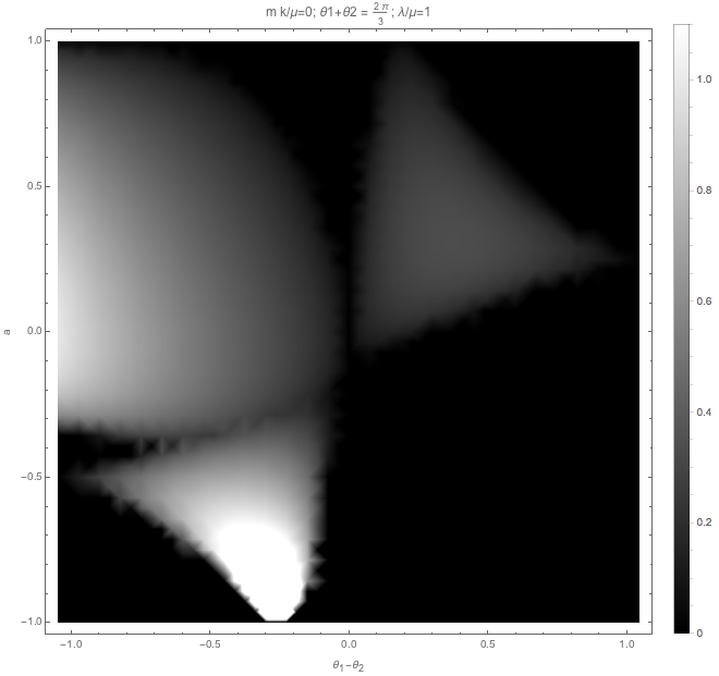
../../_images/plt2-sigmatheta-2Pi-divided-by-3-mk-divided-by-mu-0-lambda-divided-by-mu-1.png — Fig. 1.53 With matter, no vacuum frequency.¶

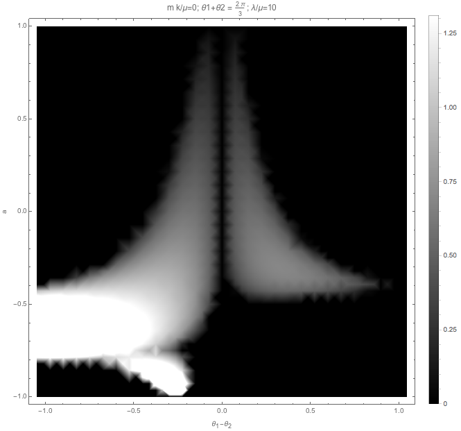
../../_images/plt2-sigmatheta-2Pi-divided-by-3-mk-divided-by-mu-0-lambda-divided-by-mu-10.png — Fig. 1.54 With matter, no vacuum frequency.¶

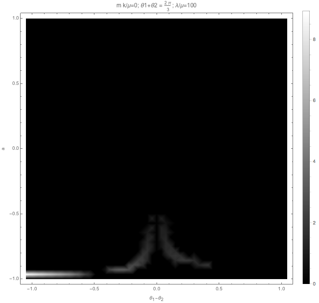
../../_images/plt2-sigmatheta-2Pi-divided-by-3-mk-divided-by-mu-0-lambda-divided-by-mu-100.png — Fig. 1.55 With matter, no vacuum frequency.¶

Then we check the result without matter, without vacuum frequency, and \(\Sigma\theta=2\pi/3\), and \(\frac{m k}{\mu}=0.1\).

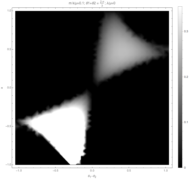
../../_images/plt2-sigmatheta-2Pi-divided-by-3-mk-divided-by-mu-0.1-lambda-divided-by-mu-0.png — Fig. 1.56 No matter, no vacuum frequency.¶

The effect of \(m k/\mu\) is also similar to matter effect.

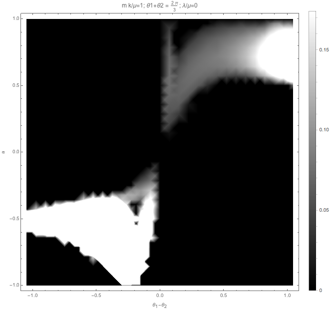
../../_images/plt2-sigmatheta-2Pi-divided-by-3-mk-divided-by-mu-1-lambda-divided-by-mu-0.png — Fig. 1.57 Higher order Fourier modes, without matter, no vacuum frequency.¶

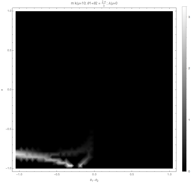
../../_images/plt2-sigmatheta-2Pi-divided-by-3-mk-divided-by-mu-10-lambda-divided-by-mu-0.png — Fig. 1.58 Higher order Fourier modes, without matter, no vacuum frequency.¶

Matter + Fourier modes also has suppression

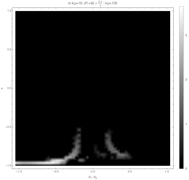
../../_images/plt2-sigmatheta-2Pi-divided-by-3-mk-divided-by-mu-10-lambda-divided-by-mu-100.png — Fig. 1.59 Higher order Fourier modes, with matter, no vacuum frequency.¶

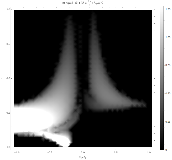
../../_images/plt2-sigmatheta-2Pi-divided-by-3-mk-divided-by-mu-1-lambda-divided-by-mu-10.png — Fig. 1.60 Higher order Fourier modes, with matter, no vacuum frequency.¶