1.3.4. Halo Effect - Analytical Methods
1.3.4.1. Linear Stability
1.3.4.1.1. Single Beam Both Start with Electron Flavor
We assume that both the forward and backward beams are starting from electron flavor.
The linearized equation of motion is
where \(\eta\) is the hierarchy and all quantities are scaled by \(\omega_v\).
We can solve the eigenvalues of this problem. To obtain complex solutions, we require \(\Delta < 0\), which translates to
where
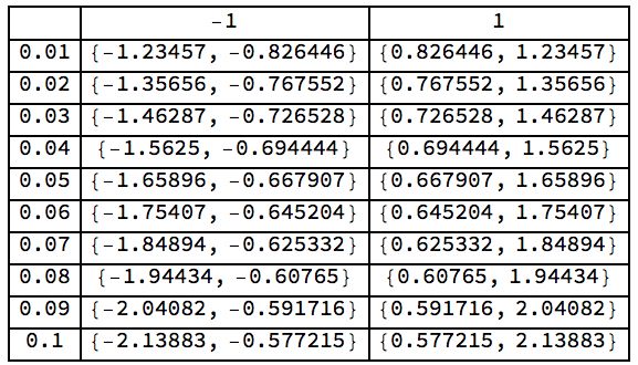
Fig. 1.182 Table of {\(\mu_{-}\), \(\mu_{+}\)}.
We plot out growth rate as a function of \(R\) and \(\mu\), which shows that such so called instabilities only exist for normal hierarchy.
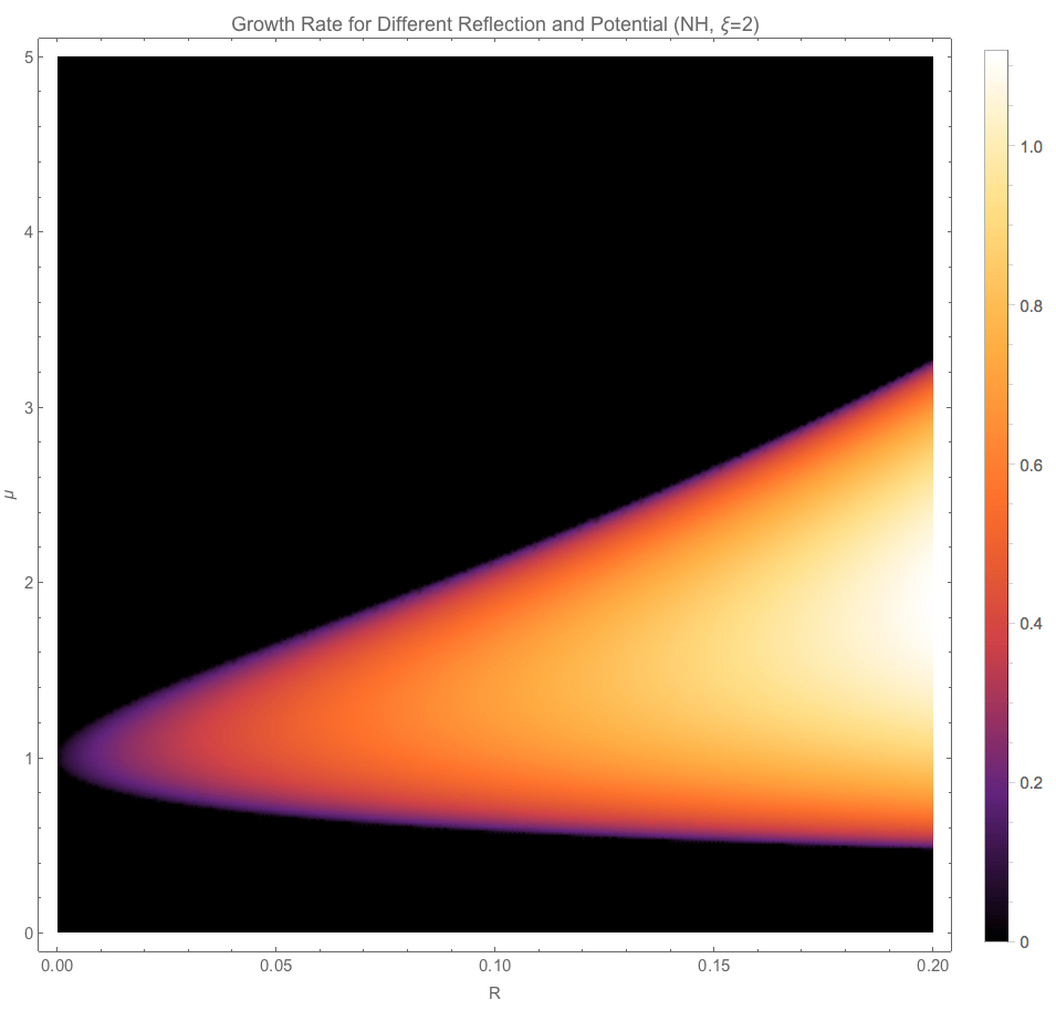
Fig. 1.183 For normal hierarchy. Vacuum mixing angle is set to 0.
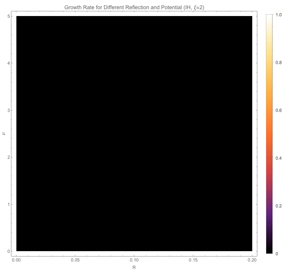
Fig. 1.184 For inverted hierarchy. Vacuum mixing angle is set to 0.
1.3.4.1.2. Single Beam Undetermined Back Beam
The equation of motion is
where
Conventions
The angle contribution is \(1-\cos\theta=2\). We absorbe this factor into \(\mu\).
As for the initial states, we can assume some general forms
The forward beam start from neutrino flavors. However, the state of the backward beam is to be determined. The exact state is not necessary since we are interested in linear stability.
We linearize the equation of motion by keeping only first order of the small off-diagonal elements.
The system of equations can be easily solved and we found that the exponentials are \(e^{i(2a R -1) \mu z}\). No exponent growth is possible.
eqnF = I D[epsF[z], z] == alpha mu (a epsF[z] - epsB[z]) + alpha mu (a epsF[z] - b)
eqnB = I D[epsB[z], z] == mu (a epsF[z] - epsB[z]) + mu (a epsF[z] - b)
DSolve[{eqnF,eqnB},{epsF,epsB},z]
The Two Beams have Synchronized Evolution
Notice that the two equations can be combined to
This result indicates that the initial development of the forward and backward beams are synchronized.
Dealing with Inhomogenous Differential Equations
The solution to inhomogenous systems is the general solution plus the particular solution. At least we can know that if the general solution contains exponential growth terms, the final solution should also contain exponential growth terms, if the particular solution doesn’t cancel them.
Floquet theory for periodic matrix systems might be useful.
1.3.4.1.2.1. Linear Regime Behavior
The solutions to such a problem shows that we always obtain decreasing modes. It’s not easy to comphrend. But the linear could be solved exactly.
In linear regime, we define the density matrices for forward and backward beams to be
The Hamiltonians are
We will investigate the instability for zero mixing angle.
The linearized equation of motion can be simplified to
This equation can be easily solved. The eigenvalues are
where
The corresponding eigenvectors are
The general solution to the equation is
The special property about this reflection prolem is that the density matrices for the forward and backward beams should be the same at the reflection point, say \(L\). With such a simple relation, we can find the relations between \(C_\pm\) by setting \(\epsilon_F(L)=\epsilon_B(L)\),
The solution to be problem can be simplified,
We are interested in the absolute values of each elements so that the overall factors can be neglected. The forward beam evolution is obtained by taking the absolute value of \(\epsilon_F\),
in which \(\sqrt{\Delta}\) is replaced by \(i \delta\).
Collecting terms, we could verify that it has the form
The only \(z\) dependent term is cosh( 2delta(L-z) ), which is decreasing within \([0,L]\) and is increasing in \([L,2L]\). The slope at \(z=L\) is 0.
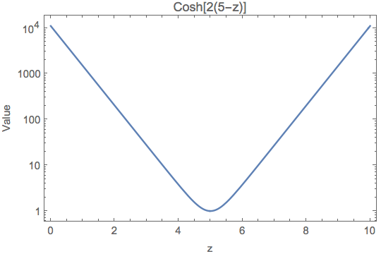
Fig. 1.185 \(\cosh(2\delta(z-L))\) with \(\delta=1\).
1.3.4.2. Nonlocal Boundary Value Problem
Some References
Springer Open has a curated list of NBVP. DENFC.
To solve coupled systems with nonlocal boundary conditions: Goodrich, C. S. (2017). Pointwise conditions in discrete boundary value problems with nonlocal boundary conditions. Applied Mathematics Letters, 67, 7–15.