1.3.1. Halo Effect - Artificial Neural Network¶

Notice

This is a summary of the work that has been done on solving vacuum oscillation using artificial neural network. Also included are some tests.

The aim of this subproject is to solve a system that could not be solved using the transitional numerical methods. The system here is a system of neutrinos emitted from a plane but interact with with the neutrinos reflected from some other plane. In this case the evolution of the emitted neutrinos are coupled to itself through the reflection.

1.3.1.1. Background¶

1.3.1.1.1. Neutrino-neutrino Interaction with The Appearance of Reflection¶

Here is the configuration.

../../_images/neutrinoWithReflection.png — Fig. 1.170 Configuration of the system. The lower plane is the emission plane while the upper plane the the reflection plane. Neutrino reaches the upper plane has a probability of being reflected, in other words there is a fixed coefficient for reflection. Only the reflected beams with angle that is the same as the emission angle are considered.¶

The lower plane is the emission plane while the upper plane the the reflection plane. Neutrinos get reflected at the upper plane with a reflection coefficient \(\alpha\). The distance between the two plane is \(d\).

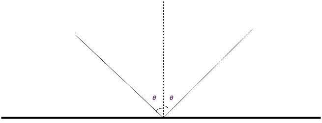
../../_images/emissionAngles.png — Fig. 1.171 There is a left-right symmetry of the emission beams. The angles are defined as \(\theta\).¶

The notation for neutrino beams are

Density Matrix of Emission to The Right: \(\rho^{Re}\)
Density Matrix of Emission to The Left: \(\rho^{Le}\)
Density Matrix of Reflection to The Right: \(\rho^{Rr}\)
Density Matrix of Reflection to The Left: \(\rho^{Lr}\)
Neutrino-neutrino Interaction of Emission to The Right: \(H_{\nu\nu}^{Re}\)
Neutrino-neutrino Interaction of Emission to The Left: \(H_{\nu\nu}^{Le}\)
Neutrino-neutrino Interaction of Reflection to The Right: \(H_{\nu\nu}^{Rr}\)
Neutrino-neutrino Interaction of Reflection to The Left: \(H_{\nu\nu}^{Lr}\)

At a fixed, each beam has a neutrino-neutrino interaction Hamiltonian with contribution from another emission beam and two reflected beams.

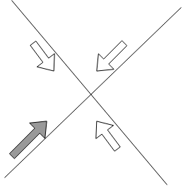
../../_images/interactionAtPoint.png — Fig. 1.172 The neutrino-neutrino interaction at a fixed point for a beam going to the right.¶

For a right emission beam, the neutrino-neutrino interaction is

\[\begin{split}H_{\nu\nu}^{Re} =& \mu \left( 2 n^{Lr} (\rho^{Lr} -\bar\rho^{Lr}) + n^{Le}(1-\cos(2\theta) ) (\rho^{Le} -\bar\rho^{Le}) \right. \nonumber \\ & \left. + n^{Rr} (1+\cos(2\theta))(\rho^{Rr} - \bar\rho^{Rr}) \right)\end{split}\]

The equation of motion for this beam is

\[i \partial_z \rho^{Re}(z) = \cos\theta \left[ H_{vac} + H_{\nu\nu}^{Re} , \rho^{Re}(z) \right],\]

where \(\hbar= c =1\).

This equation of motion shows that to calculate the evolution of the density matrix of the emission beam, we need the reflected beam, which, unfortunately depends on the emission beam. This is the reason why we tried artificial neural network. However, other methods could be found.

The other seven equation can also be written down using exactly the same trick. First of all the Hamiltonian are

\[\begin{split}H_{\nu\nu}^{Le} & = \mu \left[ 2 n^{Rr}(\rho^{Rr} - \bar \rho^{Rr}) + n^{Lr}(1+\cos 2\theta )( \rho^{Lr} - \bar \rho^{Lr} ) + n^{Re} (1-\cos 2\theta) (\rho^{Re} - \bar \rho^{Re})\right] \\ H_{\nu\nu}^{Rr}& = \mu\left[ 2 n^{Le}(\rho^{Le} - \bar \rho^{Le}) + n^{Lr} (1-\cos 2\theta)(\rho^{Lr} - \bar\rho^{Lr}) + n^{Re}(1+\cos 2\theta) (\rho^{Re} - \bar \rho^{Re}) \right] \\ H_{\nu\nu}^{Lr}& = \mu \left[ 2n^{Re}(\rho^{Re}-\bar\rho^{Re}) + n^{Rr} (1-\cos 2\theta) (\rho^{Rr} - \bar \rho^{Rr}) + n^{Le}(1+\cos 2\theta ) (\rho^{Le} - \bar \rho^{Le} ) \right]\\\end{split}\]

The EoMs are

\[\begin{split}i\partial_z \rho^{Le}(z) &= \cos\theta \left[ H_{vac} + H_{\nu\nu}^{Le}, \rho^{Le}(z) \right] \\ i\partial_z \rho^{Rr}(z) &= \cos\theta \left[ H_{vac} + H_{\nu\nu}^{Rr}, \rho^{Rr}(z) \right] \\ i\partial_z \rho^{Lr}(z) &= \cos\theta \left[ H_{vac} + H_{\nu\nu}^{Lr}, \rho^{Lr}(z) \right].\end{split}\]

For anti-neutrinos, the vacuum Hamiltonian is different from neutrinos which is \(\bar H_{vac} = - H_{vac}\). The convention is that \(z\) is always pointing up perpendicular to the emission plane.

\[\begin{split}- i \partial_z \bar \rho^{Re}(z) & = \cos\theta \left[ \bar H_{vac} + H_{\nu\nu}^{Re} , \bar \rho^{Re}(z) \right] \\ - i\partial_z \bar\rho^{Le}(z) &= \cos\theta \left[\bar H_{vac} + H_{\nu\nu}^{Le}, \bar\rho^{Le}(z) \right] \\ - i\partial_z \bar\rho^{Rr}(z) &= \cos\theta \left[\bar H_{vac} + H_{\nu\nu}^{Rr}, \bar\rho^{Rr}(z) \right] \\ - i\partial_z \bar \rho^{Lr}(z) &= \cos\theta \left[\bar H_{vac} + H_{\nu\nu}^{Lr}, \bar\rho^{Lr}(z) \right].\end{split}\]

To solve the eight first order ODEs, eight constraints are required. To begin with, all the differential equations for the emission beams are given as usual.

\[\rho^{Xe}(z=0) = \cdots ,\]

where \({}^{Xe}\) is for \({}^{Le}\) and \({}^{Re}\).

However, the other four constraints are for the reflected beams and they are not clear.

Question Here

I have a question here. Since there is no mixing between neutrinos and anti-neutrinos for Dirac particle, I would expect these constraints to be independent of each other. Is this true?

\[\begin{split}\rho^{Lr}(z=d) & = \mathbf{Refl} [\rho^{Le}(z=d)] \\ \rho^{Rr}(z=d) & = \mathbf{Refl} [ \rho^{Rr}(z=d) ] \\ \bar\rho^{Lr}(z=d) & = \mathbf{Refl} [\bar \rho^{Le}(z=d)] \\ \bar \rho^{Rr}(z=d) & = \mathbf{Refl} [ \bar \rho^{Re}(z=d)],\end{split}\]

in which \(\mathbf{Refl}\) is the operator for the reflection that takes out some of the diagonal elements and multiplied each element by a constant.

Question

The question is how to determine this \(\mathbf{Refl}\)

1.3.1.2. Numerical Methods¶

1.3.1.2.1. Artificial Neural Network for Vacuum Oscillation¶

To make sure artificial neural network actually works, we started from the calculation of vacuum oscillation. In this section we consider only two flavour neutrino oscillation.

1.3.1.2.1.1. Vacuum Oscillation¶

Neutrino Vacuum Oscillation is determined by the following equation of motion.

\[i\partial_t \rho = \left[ H_{vac},\rho \right],\]

where \(\rho\) is the density matrix and can be written as

\[\begin{split}\rho = \begin{pmatrix} a & b + i c\\ b - i c & d \end{pmatrix},\end{split}\]

in which all the \(a,b,c,d\) are real.

The vacuum Hamiltonian is

\[\begin{split}H_{vac} = \frac{\delta^2 m}{4 E}\begin{pmatrix} -\cos(2\theta_v) & \sin(2\theta_v)\\ \sin(2\theta_v) & \cos(2\theta_v)\end{pmatrix}.\end{split}\]

Plug in this vacuum Hamiltonian we can write down four equations for \(a,b,c,d\).

Suppose we can write the vacuum Hamiltonian as

\[\begin{split}H_{vac} = \begin{pmatrix} h0 & h1 \\ h2 & h3 \end{pmatrix}.\end{split}\]

Von Neumann equation shows that

\[i \partial_t \rho = \left[ H_{vac}, \rho \right],\]

Using the previous notations, I find four equations

\[\begin{split}\dot a &= - (h1+h2) c \\ \dot b &= (h0-h3) c \\ \dot c &= a ~ h1 + d~h1 + b (h0-h3) \\ \dot d & = c (h0-h3).\end{split}\]

There are two ways of writing the program.

2 by 2 Matrix
1 by 4 Matrix

In this note, we will use a 1 by 4 matrix to denote the density matrix, which is defined as,

\[\begin{split}\rho = \begin{pmatrix} a \\ d \\ b \\ c \end{pmatrix}\end{split}\]

The equation of motion becomes

\[\begin{split}\partial_t \begin{pmatrix} a \\ d \\ b \\ c \end{pmatrix} = \begin{pmatrix} - (h1+h2) c \\ (h0-h3) c \\ a~h1 + d~h1 + b (h0-h3) \\ c (h0-h3) \end{pmatrix}\end{split}\]

For vacuum oscillations, the Hamiltonian is

\[\begin{split}H_{vac} \propto \begin{pmatrix} -\cos 2\theta & \sin 2\theta \\ \sin 2\theta & \cos 2\theta \end{pmatrix},\end{split}\]

which leads to

\[\begin{split}\partial_t \begin{pmatrix} a \\ d \\ b \\ c \end{pmatrix} = \begin{pmatrix} - 2 c \sin 2\theta \\ -2c \cos 2\theta \\ a\sin 2\theta + d \sin 2\theta - 2b \cos 2\theta \\ -2c\cos 2\theta \end{pmatrix}.\end{split}\]

The four equations can be solved and the density matrix at any time can be obtained.

1.3.1.2.1.2. Artificial Neural Network for Vacuum Oscillation¶

The code I have been testing is written by Shashank for my code doesn’t minimized to a good result.But the debugging for my code is also shown below.

Debugging( Compare my code with Shashank’s code)

My code can also be found here at nbviewer .

Through the debugging I have confirmed that we have the same function value given the same arguments and the same cost function value in the same condition. But my code doesn’t show a good minimization result.

Testing ANN for Vacuum Oscillation using Shashank’s Code

These are tests done using Shashank’s code. Three types of tests has been done.

Using only Nelder-Mead

vout=minimize(yp,partot,method='Nelder-Mead',tol=1e-11,
options={"ftol":1e-9, "maxfev": 100000000,"maxiter":1000000000})

The result appears to be not bad. (“nfev”: number of function evaluation; “nit”: number of total iterations.)

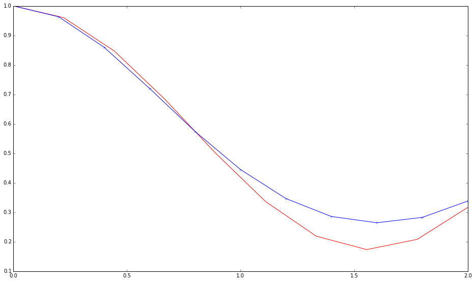
../../_images/ann_NelderMead.png — Fig. 1.173 The 11 element of density matrix as a function of time. The red curve is accurate result while the blue is the numerical one.¶

status: 0
nfev: 145333
success: True
fun: 0.08876848018538129
x: array([ 1.21427619, 2.79927002, -0.31095306, -3.03716024, 0.56912385,
0.58925948, -2.20871918, -0.4288958 , -0.32492061, 0.49362869, 0.58244097,
-0.22038025, -0.1011485 , 0.52798698, -2.32437879, 0.44040058, 0.38382487,
0.55826206, -4.94480949, -1.07137694, 4.11333683, -1.50943871, 2.71204262,
-0.76276552, 1.55497648, 0.22475994, 0.88421604, -1.06671129, -2.00532868,
-3.00326507, 0.48030015, 0.25948442, 0.25845743, -0.82423628, 0.78934658,
0.39508506, 0.02805506, -0.02669909, 10.68427395, -1.4504223 , -3.26192936,
7.52701912, -2.55832534, 4.79891183, 4.44328441, -0.14572288, -0.59159877,
0.23857354, -4.99080565, 3.47041765, -2.27428677, -1.07234212, 1.76593101,
-2.21089853, -2.83558577, -0.94328398, -1.99377883, -2.21098883, 0.38034013,
0.43636049])
message: 'Optimization terminated successfully.'
nit: 131078

Using Only Differential Evolution

For a range of time in (0,2),

x=np.linspace(0,2,11)

and using only differential evolution,

vout=differential_evolution(yp,bounds,strategy='best1bin',tol=0.1, maxiter=100, polish=True)

the function result turns out to be,

5.649973778537050774e-03

while the result for x array is

[-0.46752427 -2.65884641 -0.87100392 2.21847349 -0.68876981
-1.18718098 -2.45899394 -2.41608376 -2.03016303 -2.50621246
-1.72752687 -3.52288081 4.53627758 -0.11251283 -2.78713549
-0.44748985 1.64193553 -0.92174658 -0.99302148 1.09775197
-1.17935884 -1.71925608 -2.83591163 -0.52258003 -2.71429398
1.35386314 3.34156037 0.96810593 0.24346204 -4.39480932 2.09637481
-0.74179975 3.26104658 -2.72595898 -0.76631589 -2.21640847
-3.25833908 -0.78663055 -1.55206952 0.46654166 -4.8803229
-4.26865044 -0.12565569 0.10469799 -1.8695357 -0.15555892
-1.17371098 0.26577405 0.875804 -2.51542228 -4.29488662 -2.6605975
1.96894693 -3.09901811 -1.39401083 0.96014599 2.95403418
3.79841345 -2.10529717 -4.10821308]

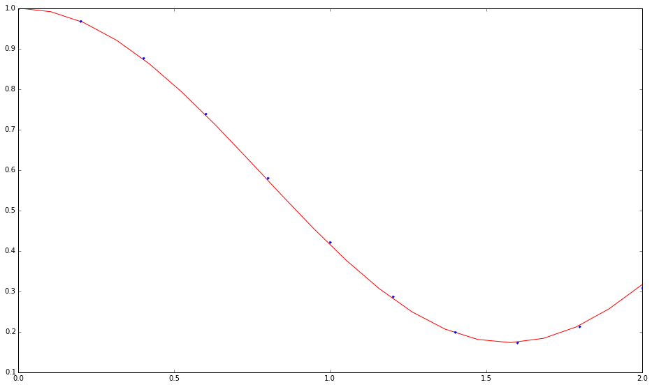
../../_images/ann_devo.png — Fig. 1.174 The 11 element of density matrix as a function of time. The red curve is accurate result while the blue is from differential evolution.¶

Calculating a Longer Range

Double the range to

x=np.linspace(0,4,11)

and apply only differential evolution.

vout=differential_evolution(yp,bounds,strategy='best1bin',tol=0.01, maxiter=1000,polish=True)

The result is very bad.

nfev: 105906
success: False
fun: 0.15264565359933352
x: array([ 1.2415797 , -1.27267036, 0.14521048, 1.06534837, -0.22554095,
1.97210186, 4.85844909, -1.5015446 , -2.66713337, -0.59127114, -1.17100097,
0.72691612, -3.84768313, 0.68169926, 1.61422628, -1.69251485, 0.61827763,
-1.70389394, -2.90578576, 4.69827117, -4.18291259, -1.74349331, 3.76258326,
0.95722587, 5. , 2.80036916, -4.24126024, -2.45899517, 0.99396641, 1.54324845,
-2.99045871, -0.26770419, 1.62076744, -3.41084945, -1.31280928, -2.21778869,
2.4837208 , 2.81803398, -3.94093507, 1.63757038, -3.5154411 , 2.93116174,
0.74082291, -3.26617915, -0.19332002, 1.75131816, -1.46409058, 2.342905 ,
-1.78805522, -2.55208371, -3.55389878, -3.7073305 , -1.98135275, -3.88337902,
-3.3127076 , 0.13548304, 1.90006674, -3.89693459, -1.37139011, -2.28290761])
message: 'Maximum number of iterations has been exceeded.'
jac: array([ 9.90042492e-02, 9.56093427e-02, 5.69877479e-05, 9.94637706e-04,
3.43239936e-02, 4.57047178e-03, -1.29582733e-03, 2.14828155e-06,
-4.48536763e-03, -1.63860814e-02, -2.19701479e-03, -4.18309276e-03,
8.10185252e-06, -4.03330425e-03, -4.40266712e-03, -9.43032319e-03,
-1.44689816e-04, -1.15090820e-01, -1.20024951e-01, -1.24700941e-01,
-1.07455711e-03, -1.56707980e-05, -3.08311154e-03, 2.43753712e-02,
-3.95701805e-03, -5.22216714e-03, -8.87512286e-05, -5.17548226e-03,
1.23602240e-02, -4.17025858e-03, 4.53925786e-04, -6.57369575e-02,
-6.92782415e-02, 4.67753614e-04, -7.70130126e-02, -3.59692831e-04,
-5.45286039e-05, 3.42913198e-03, 1.46133106e-04, 7.60768115e-03,
-1.32331091e-03, -1.87794225e-04, 5.21242494e-03, -1.47535317e-03,
-8.97968366e-03, 3.09193504e-03, -7.49011964e-05, -2.00667261e-04,
1.80120363e-03, 7.68457520e-04, -2.31557273e-03, -1.89914195e-03,
-2.09954831e-03, 6.48930909e-04, 7.02615743e-04, 4.39465131e-04,
4.34813574e-03, -4.79563611e-04, -2.18436380e-03, -1.66073266e-03])
nit: 100

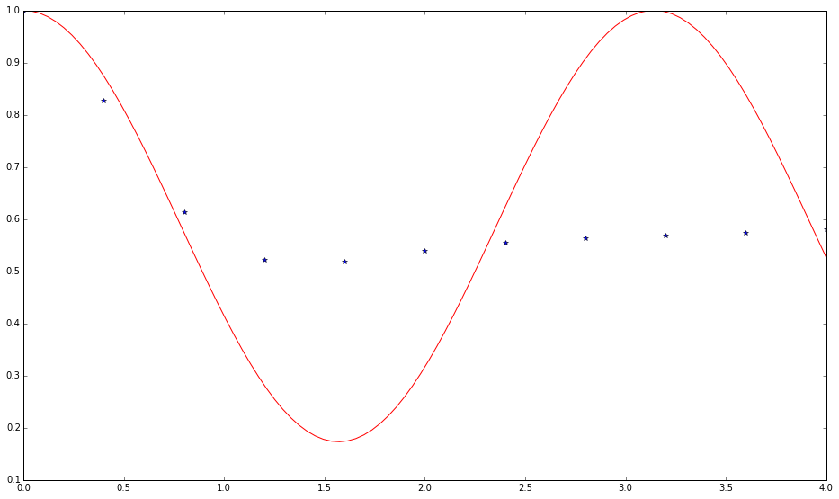
../../_images/ann_devo_range.png — Fig. 1.175 The 11 element of density matrix as a function of time. The red curve is accurate result while the blue is from differential evolution.¶

1.3.1.2.2. Codes¶

import numpy as np
from scipy.optimize import minimize
from scipy.special import expit
import matplotlib.pyplot as plt
import scipy
from matplotlib.lines import Line2D
import timeit
import pandas as pd

array12 = np.asarray(np.split(np.random.rand(1,60)[0],12))

def act(x):
    return expit(x)

# Density matrix in the forms that I wrote down on my Neutrino Physics notebook
# x is a real array of 12 arrays.

init = np.array([1.0,0.0,0.0,0.0])

def rho(x,ti,initialCondition):

    elem = np.ones(4)

    for i in np.linspace(0,3,4):
        elem[i] = np.sum(ti*x[i*3]*act(ti*x[i*3+1] + x[i*3+2]) )

    return init + elem

rho(array12,0,init)

hamil = np.array( [  np.cos(2.0),np.sin(2.0) , np.sin(2.0),np.cos(2.0) ] )
print hamil

def rhop(x,ti,initialCondition):

    rhoprime = np.zeros(4)

    for i in np.linspace(0,3,4):
        rhoprime[i] = np.sum(x[i*3] * (act(ti*x[i*3+1] + x[i*3+2]) ) ) +  np.sum( ti*x[i*3]* (act(ti*x[i*3+1] + x[i*3+2]) ) * (1.0 - (act(ti*x[i*3+1] + x[i*3+2])  ) )* x[i*3+1]  )

    return rhoprime

## This is the regularization which is not used in this code

regularization = 0.0001

def costi(x,ti,initialCondition):

    rhoi = rho(x,ti,initialCondition)
    rhopi = rhop(x,ti,initialCondition)

    costTemp = np.zeros(4)

    costTemp[0] = ( rhopi[0] - 2.0*rhoi[3]*hamil[1] )**2
    costTemp[1] = ( rhopi[1] + 2.0*rhoi[3]*hamil[1] )**2
    costTemp[2] = ( rhopi[2] - 2.0*rhoi[3]*hamil[0] )**2
    costTemp[3] = ( rhopi[3] + 2.0*rhoi[2]*hamil[0] - hamil[1] * (rhoi[1] - rhoi[0] ) )**2

    return np.sum(costTemp)# + 2.0*(rhoi[0]+rhoi[1]-1.0)**2

#    return np.sum(costTemp) + regularization*np.sum(x**2)

costi(array12,0,init)

def cost(x,t,initialCondition):

    costTotal = map(lambda t: costi(x,t,initialCondition),t)

    return 0.5*np.sum(costTotal)

cost(array12,np.array([0,1,2]),init)
#cost(xresult,np.array([0,4,11]),init)

# initGuess = np.asarray(np.split( 5.0*(np.random.rand(1,60)[0] - 0.5),12))
initGuess = np.split(np.zeros(60),12)
endpoint = 2
tlin = np.linspace(0,endpoint,11)

costF = lambda x: cost(x,tlin,init)

start = timeit.default_timer()
costvFResult = minimize(costF,initGuess,method='Nelder-Mead',tol=1e-5,options={"ftol":1e-3, "maxfev": 10000000,"maxiter":10000000})
stop = timeit.default_timer()

print stop - start
timespent = stop - start

print costvFResult

xresult = costvFResult.get("x")

print xresult

#np.savetxt('costvFResult.txt',costvFResult,delimiter=',')

np.savetxt('xresult.txt', xresult, delimiter = ',')

np.savetxt('timespent.txt', np.array([timespent]), delimiter = ',')

np.savetxt('functionvalue.txt', np.array([costvFResult.fun]), delimiter=',')