1.1.4. Single Frequency Matter Perturbation¶

As a first step, we solve single frequency matter perturbation

δ λ (x) = A \sin (k x + ϕ) .

Using the relation between $η$ and $δ λ$ , we solve out $η$ .

η (x) = - \frac{ω_{m}}{2} x - \frac{\cos 2 θ_{m}}{2} \frac{A}{k} \cos (k x + ϕ),

where we have chosen $η (0) = - \frac{\cos 2 θ_{m}}{2} \frac{A}{k} \cos ϕ$ .

The problem is to solve the equation of motion

\begin{array}{r} i \frac{d}{d x} (\begin{array}{c} ψ_{b 1} \\ ψ_{b 2} \end{array}) = \frac{\sin 2 θ_{m}}{2} δ λ (x) (\begin{array}{c} 0 & e^{2 i η (x)} \\ e^{- 2 i η (x)} & 0 \end{array}) (\begin{array}{c} ψ_{b 1} \\ ψ_{b 2} \end{array}) . \end{array}

We also define

(1.10)¶

\begin{aligned} h & = \frac{\sin 2 θ_{m}}{2} δ λ (x) e^{2 i η (x)} \\ = \frac{\sin 2 θ_{m}}{2} A \sin (k x + ϕ) e^{i (- ω_{m} x - \frac{A \cos 2 θ_{m}}{k} \cos (k x + ϕ))}, \end{aligned}

so that the equation of motion becomes

\begin{array}{r} i \frac{d}{d x} (\begin{array}{c} ψ_{b 1} \\ ψ_{b 2} \end{array}) = (\begin{array}{c} 0 & h \\ h^{*} & 0 \end{array}) (\begin{array}{c} ψ_{b 1} \\ ψ_{b 2} \end{array}) . \end{array}

Obviously, the exponential terms is too complicate. On the other hand, this equation of motion reminds us of the Rabi oscillation. So we decide to rewrite the exponential into some plane wave terms using Jacobi-Anger expansion. (Refs & Notes: Patton et al)

Jacobi-Anger Expansion

One of the forms of Jacobi-Anger expansion is

(1.11)¶

e^{i z \cos (Φ)} = \sum_{n = - \infty}^{\infty} i^{n} J_{n} (z) e^{i n Φ} .

We define $z_{k} = \frac{A}{k} \cos 2 θ_{m}$ , with which we expand the term

e^{- i \frac{\cos 2 θ_{m} A}{k} \cos (k x + ϕ)} = \sum_{n = - \infty}^{\infty} i^{n} J_{n} (- z_{k}) e^{i n (k x + ϕ)} = \sum_{n = - \infty}^{\infty} (- i)^{n} J_{n} (z_{k}) e^{i n (k x + ϕ)},

where I used $J_{n} (- z_{k}) = (- 1)^{n} J_{n} (z_{k})$ for integer $n$ .

The expansion is plugged into the Hamiltonian elements,

\begin{aligned} h & = \frac{A \sin 2 θ_{m} \sin (k x + ϕ)}{2} e^{- i ω_{m} x} \sum_{n = - \infty}^{\infty} (- i)^{n} J_{n} (z_{k}) e^{i n (k x + ϕ)} \\ = \frac{A \sin 2 θ_{m}}{4 i} (e^{i (k x + ϕ)} - e^{- i (k x + ϕ)}) e^{- i ω_{m} x} \sum_{n = - \infty}^{\infty} (- i)^{n} J_{n} (z_{k}) e^{i n (k x + ϕ)} \\ = \frac{A \sin 2 θ_{m}}{4 i} (\sum_{n = - \infty}^{\infty} e^{i (n + 1)} i^{n} J_{n} (z_{k}) e^{i ((n + 1) k - ω_{m}) x} - \sum_{n^{'} = - \infty}^{\infty} e^{i (n^{'} - 1)} (- i)^{n^{'}} J_{n^{'}} (z_{k}) e^{i ((n^{'} - 1) k - ω_{m}) x}) \\ = \frac{A \sin 2 θ_{m}}{4} \sum_{n = - \infty}^{\infty} e^{i n ϕ} (- (- i)^{n}) \frac{2 n}{z_{k}} J_{n} (z_{k}) e^{i (n k - ω_{m}) x}, \end{aligned}

where I have used

J_{n - 1} (z_{k}) + J_{n + 1} (z_{k}) = \frac{2 n}{z_{k}} J_{n} (z_{k}) .

Here comes the approximation. The most important oscillation we need is the one with largest period, which indicates the phase to be almost zero,

(1.12)¶

\begin{aligned} (n + 1) k - ω_{m} & \sim 0 \\ (n^{'} - 1) k - ω_{m} & \sim 0. \end{aligned}

The two such conditions for the two summations are

\begin{aligned} n \equiv n_{-} & = Int (\frac{ω_{m}}{k}) - 1 \\ n^{'} \equiv n_{+} & = Int (\frac{ω_{m}}{k}) + 1 . \end{aligned}

We define $Int (\frac{ω_{m}}{k}) = n_{0}$ ,

\begin{aligned} n_{-} & = n_{0} - 1 \\ n_{+} & = n_{0} + 1 . \end{aligned}

The element of Hamiltonian is written as

h = - \frac{A \sin 2 θ_{m}}{2} e^{i n_{0} ϕ} (- i)^{n_{0}} \frac{n_{0}}{z_{k}} J_{n_{0}} (z_{k}) e^{i (n_{0} k - ω_{m}) x} .

To save keystrokes, we define

(1.13)¶

F = - A \sin 2 θ_{m} e^{i n_{0} ϕ} (- i)^{n_{0}} \frac{n_{0}}{z_{k}} J_{n_{0}} (z_{k}),

which depends on $n_{0}$ and $z_{k} = \frac{A}{k} \cos 2 θ_{m}$ . Notice that

| F |^{2} = {| k \tan 2 θ_{m} n_{0} J_{n_{0}} (z_{k}) |}^{2} .

Thus the 12 element of the Hamiltonian is rewritten as

(1.14)¶

h = \frac{1}{2} F e^{i (n_{0} k - ω_{m}) x} .

Solving Using Mathematica

The Mathematica code:

In[1]:= sys = I D[{phi1[x], phi2[x]}, x] == {{0, (g0R + I g0I) Exp[ I (-omegam + n0 k) x]}, {(g0R - I g0I) Exp[-I (-omegam + n0 k) x], 0}}.{phi1[x], phi2[x]}
In[2]:= DSolve[sys, {phi1, phi2}, x]// FullSimplify
Out[3]:= {{phi1 -> Function[{x},
E^(1/2 I (k n0 + I Sqrt[-4 (g0I^2 + g0R^2) - (k n0 - omegam)^2] - omegam) x) C[1]
+ E^(1/2 (Sqrt[-4 (g0I^2 + g0R^2) - (k n0 - omegam)^2] + I (k n0 - omegam)) x) C[2]],
phi2 -> Function[{x}, (1/(2 (g0I - I g0R)))
I E^(-I (k n0 - omegam) x +
 1/2 I (k n0 + I Sqrt[-4 (g0I^2 + g0R^2) - (k n0 - omegam)^2] - omegam) x)
 (k n0 + I Sqrt[-4 (g0I^2 + g0R^2) - (k n0 - omegam)^2] - omegam) C[1]
 + (1/(2 (g0I - I g0R))) E^(1/2 (Sqrt[-4 (g0I^2 + g0R^2) - (k n0 - omegam)^2]
 + I (k n0 - omegam)) x - I (k n0 - omegam) x) (Sqrt[-4 (g0I^2 + g0R^2) - (k n0 - omegam)^2]
 + I (k n0 - omegam)) C[2]]}}

The general solution to the equation of motion is

\begin{aligned} ψ_{b 1} = & C_{1} e^{\frac{1}{2} i (n_{0} k - ω_{m} - \sqrt{| F |^{2} + (n_{0} k - ω_{m})^{2}}) x} + C_{2} e^{\frac{1}{2} i (n_{0} k - ω_{m} + \sqrt{| F |^{2} + (n_{0} k - ω_{m})^{2}}) x} \\ ψ_{b 2} = & \frac{C_{1}}{F^{*}} i (n_{0} k - ω_{m} - \sqrt{| F |^{2} + (n_{0} k - ω_{m})^{2}}) e^{- \frac{1}{2} i (n_{0} k - ω_{m}) x - \frac{1}{2} i \sqrt{| F |^{2} + (n_{0} k - ω_{m})^{2}}} \\ + \frac{C_{2}}{F^{*}} i (n_{0} k - ω_{m} + \sqrt{| F |^{2} + (n_{0} k - ω_{m})^{2}}) e^{- \frac{1}{2} i (n_{0} k - ω_{m}) x + \frac{1}{2} i \sqrt{| F |^{2} + (n_{0} k - ω_{m})^{2}}} . \end{aligned}

For simplicity, we define

(1.15)¶

\begin{aligned} g & = n_{0} k - ω_{m}, \\ q^{2} & = | F |^{2} + g^{2} . \end{aligned}

To determine the constants, we need intial condition,

\begin{array}{r} (\begin{array}{c} ψ_{1} (0) \\ ψ_{2} (0) \end{array}) = (\begin{array}{c} 1 \\ 0 \end{array}), \end{array}

which leads to

\begin{array}{r} (\begin{array}{c} ψ_{b 1} (0) \\ ψ_{b 2} (0) \end{array}) = (\begin{array}{c} e^{i η (0)} \\ 0 \end{array}), \end{array}

using equation wavefunction in background matter basis.

Plug in the initial condition for the wave function,

\begin{aligned} C_{1} + C_{2} & = e^{i \frac{z_{k}}{2} \cos ϕ} \\ \frac{C_{1}}{2 F^{*}} i (g - q) + \frac{C_{2}}{F^{*}} i (q + g) & = 0. \end{aligned}

The constants are solved out

\begin{aligned} C_{1} & = e^{i \frac{z_{k}}{2} \cos ϕ} \frac{q + g}{2 q}, \\ C_{2} & = e^{i \frac{z_{k}}{2} \cos ϕ} \frac{q - g}{2 q} . \end{aligned}

where $F$ is defined in (1.13) and $l$ and $g$ are defined in (1.15).

The second element of wave function becomes

ψ_{b 2} (x) = \frac{- F}{q} e^{i \frac{z_{k}}{2} \cos ϕ} e^{- \frac{i}{2} g x} \sin (\frac{1}{2} q x) .

The transition probability becomes

P_{1 \to 2} = | ψ_{b 2} |^{2} = \frac{| F |^{2}}{q^{2}} \sin^{2} (\frac{q}{2} x),

where $q$ is the oscillation wavenumber. Period of this oscillation is given by $T = \frac{2 π}{q}$ .

Compare The Result with Kneller et al

Kneller et al have a transition probability

P_{12} = \frac{κ_{n}^{2}}{q_{n}^{2}} \sin^{2} (q_{n} x),

where $q_{n}^{2} = k_{n}^{2} + κ_{n}^{2}$ and $2 k_{n} = {\tilde{δ k}}_{12} + n k_{⋆}$ .

In my notation, $k$ is the same as their $k_{⋆}$ . After the first step of translation, we have $g = 2 k_{n}$ .

The definition of $κ_{n}$ is given by

in Kneller’s notation and

δ V_{e e} (x) = C_{⋆} V_{⋆} \sin (k_{⋆} x + η) .

So we conclude that my $| F |^{2}$ is related to Kneller’s $| κ_{n} |^{2}$ through

| F |^{2} = 4 | κ_{n} |^{2} .

We also have

q^{2} = | F |^{2} + g^{2} = 4 q_{n}^{2},

i.e., $q_{n} = \frac{q}{2}$ .

Now we see the method we have used gives exactly the same transition probability as Kneller’s.

To make the numerical calculations easier, we rewrite the result by defining the scaled variables

\begin{aligned} \hat{x} & = ω_{m} x, \\ \hat{k} & = \frac{k}{ω_{m}}, \\ \hat{A} & = \frac{A}{ω_{m}}, \\ \hat{g} & = \frac{g}{ω_{m}} = n_{0} \hat{k} - 1, \\ \hat{q} & = \sqrt{| \hat{F} |^{2} + {\hat{g}}^{2}} = \sqrt{| \hat{k} \tan 2 θ_{m} n_{0} J_{n_{0}} (z_{k}) | + {\hat{g}}^{2}}, \end{aligned}

so that $n_{0} = Round (1 / \hat{k})$ , $z_{k} = \frac{\hat{A}}{\hat{k}} \cos 2 θ_{m}$ and

(1.16)¶

P_{1 \to 2} = \frac{{| \hat{k} \tan 2 θ_{m} n_{0} J_{n_{0}} (z_{k}) |}^{2}}{{| \hat{k} \tan 2 θ_{m} n_{0} J_{n_{0}} (z_{k}) |}^{2} + {\hat{g}}^{2}} \sin^{2} (\frac{\hat{q}}{2} \hat{x}) .

1.1.4.1. Mathematical Analysis of The Result¶

There are several question to answer before we can understand the picture of the math.

What does each term mean in the Hamiltonian?
What exactly is the unitary transformation we used to rotate the wave function?
What is the physical meaning of Jacobi-Anger expansion in our calculation?

To answer the first question, we need to write down the solution to Schrodinger equation assuming the Hamiltonian has only one term. The results are listed below.

Hamiltonian	Solution to The First Element of Wave Function
$- \frac{ω_{m}}{2} σ_{3}$	$ψ_{1} \sim e^{i ω_{m} x / 2}$
$\frac{δ λ}{2} \cos 2 θ_{m} σ_{3}$	$ψ_{1} \sim e^{i \frac{A \cos 2 θ_{m}}{2 k} \cos (k x + ϕ)}$
$\frac{δ λ}{2} \cos 2 θ_{m} σ_{3}$	$ψ_{1} = C_{1} e^{i \frac{A \sin 2 θ_{m}}{2 k} \cos (k x + ϕ)} + C_{2} e^{- i \frac{A \sin 2 θ_{m}}{2 k} \cos (k x + ϕ)}$

The unitary transformation used is to move our reference frame to a co-rotating one. $- \frac{ω_{m}}{2} σ_{3}$ is indeed causing the wave function to rotate and removing this term using a transformation means we are co-rotating with it. $\frac{δ λ}{2} \cos 2 θ_{m} σ_{3}$ causes a more complicated rotation however it is still a rotation.

As for Jacobi-Anger expansion, it expands an oscillating matter profile to infinite constant matter potentials. To see it more clearly, we assume that $δ λ = λ_{c}$ is constant. After the unitary transformation, the effective Hamiltonian is

\begin{array}{r} H^{'} = \frac{\sin 2 θ_{m}}{2} λ_{c} (\begin{array}{c} 0 & e^{2 i η (x)} \\ e^{- 2 i η (x)} & 0 \end{array}), \end{array}

where $η (x) = - \frac{ω_{m}}{2} x + \frac{\cos 2 θ_{m}}{2} λ_{c} x$ and we have chosen $η (0) = 0$ .

The 12 element of the Hamiltonian becomes

\frac{\sin 2 θ_{m}}{2} λ_{c} e^{2 i η (x)} = \frac{\sin 2 θ_{m}}{2} λ_{c} e^{2 i (\frac{ω_{m}}{2} + \frac{\cos 2 θ_{m}}{2} λ_{c}) x} .

The significance of it is to show that a constant matter profile will result in a simple exponential term. However, as we move on to periodic matter profile, we have a Hamiltonian element of the form

h = \frac{\sin 2 θ_{m}}{2} A \sin (k x + ϕ) e^{2 i (- \frac{ω_{m}}{2} x + \frac{A \cos 2 θ_{m}}{2 k} \cos (k x + ϕ))},

as derived in equation (1.10). To compare with the constant matter case, we make a table of relevant terms in Hamiltonian.

Constant Matter Profile $δ λ = λ_{c}$	Period Matter Profile $δ λ = A \sin (k x + ϕ)$
$\frac{\sin 2 θ_{m}}{2} λ_{c} e^{i \cos 2 θ_{m} λ_{c} x}$	$\frac{A \sin 2 θ_{m}}{4} \sum_{n = - \infty}^{\infty} e^{i n ϕ} (- i^{n}) \frac{2 n + 1}{z_{k}} J_{n} (z_{k}) e^{i (n k - ω_{m}) x}$

The periodic profile comes into the exponential. Jacobi-Anger expansion (equation (1.11)) expands the periodic matter profile into infinite constant matter profiles. By comparing the two cases, we conclude that $\cos 2 θ_{m} λ_{c}$ corresponds to $n k$ .

The RWA approximation we used to drop fast oscillatory terms in the summation is to find the most relevant constant matter profile per se.

The big question is which constant matter profiles are the most important ones? Mathematically, we require the phase to be almost zero, i.e. equation (1.12) or

n_{0} k - ω_{m} \sim 0,

where $n_{0} = Round (\frac{ω_{m}}{k})$ .

What is the meaning of this condition in this new basis? If we define a effective matter density out of the Jacobi-Anger expanded series, we should define it to be

λ_{c}^{'} = \frac{n_{0} k}{\cos 2 θ_{m}} .

Then we can rewrite the RWA requirement as

λ_{c}^{'} - \cos 2 θ_{m} ω_{m} = 0.

A Reminder of MSW Resonance

The MSW Hamiltonian in flavor basis is

H = \frac{ω_{v}}{2} (- \cos 2 θ_{v} σ_{3} + \sin 2 θ_{v} σ_{1}) + \frac{λ}{2} σ_{3} + Δ I,

where the MSW resonance happens when all the $σ_{3}$ terms cancel eath other, i.e.,

- ω_{v} \cos 2 θ_{v} + λ = 0.

1.1.4.2. The Resonances¶

Questions

There are several questions to be answered.

How good is the RWA approximation? What are the conditions?
What can we use for other calculations?
Multiple matter frequency?

Now we check the Hamiltonian again to see if we could locate some physics. In the newly defined basis and using scaled quantities

\begin{array}{r} \hat{H} = (\begin{array}{c} 0 & \hat{h} \\ {\hat{h}}^{*} & 0 \end{array}), \end{array}

where

\hat{h} = \frac{1}{2} {\hat{B}}_{n} e^{i (n \hat{k} - 1) \hat{x}},

and

{\hat{B}}_{n} = (- i)^{n} \hat{k} \tan 2 θ_{m} n J_{n} (\frac{\hat{A}}{\hat{k}} \cos 2 θ_{m}) .

It becomes much more clearer if we plug $\hat{h}$ back into Hamiltonian. What we find is that

\begin{array}{r} \hat{H} = \sum_{n = - \infty}^{\infty} (\begin{array}{c} 0 & - \frac{1}{2} {\hat{B}}_{n} e^{i (n \hat{k} - 1) \hat{x}} \\ - \frac{1}{2} {\hat{B}}_{n}^{*} e^{- i (n \hat{k} - 1) \hat{x}} & 0 \end{array}) . \end{array}

With some effort, we find that the solution to the second amplitude of the wave function is

ψ_{2} = \frac{i}{{\hat{B}}_{n} \hat{W}} e^{- i (n \hat{k} - 1) \hat{x}} {| {\hat{B}}_{n} |}^{2} \sin (\frac{1}{2} (n \hat{k} - 1 - \hat{W}) \hat{x}),

where

\hat{W} = \sqrt{(n \hat{k} - 1)^{2} + {| {\hat{B}}_{n} |}^{2}} .

At this stage, it is quite obvious that our system is a composite Rabi oscilation system. For each specific $n$ term we write down the hopping probability from light state to the heavy state,

P_{L \to H}^{(n)} = \frac{{| {\hat{B}}_{n} |}^{2}}{{| {\hat{B}}_{n} |}^{2} + (n \hat{k} - 1)^{2}} \sin^{2} (\frac{{\hat{q}}^{(n)}}{2} \hat{x}),

where

\begin{aligned} Γ^{(n)} & = | {\hat{B}}_{n} |, width of resonance (n \hat{k} as parameter) \\ {\hat{q}}^{(n)} & = \sqrt{{| Γ^{(n)} |}^{2} + (n \hat{k} - 1)^{2}}, frequency of oscillations \end{aligned}

Scaled Quantities

As a reminder, the scaled quantities are defined as

\begin{aligned} \hat{x} & = ω_{m} x, \\ \hat{h} & = h / ω_{m}, \\ {\hat{B}}_{n} & = B_{n} / ω_{m}, \\ \hat{k} & = k / ω_{m}, \\ \hat{A} & = A / ω_{m}, \\ \hat{q} & = q / ω_{m} . \end{aligned}

Just a comment. $B_{n}$ is used here because I actually want to use it for multi-frequency case and I just think $B_{n}$ is better than $F$ .

Rabi Oscillations

The form of Hamiltonian reminds of us Rabi oscillations, whose Hamiltonian is

\begin{array}{r} (\begin{array}{c} - ω_{0} / 2 & α ω_{0} e^{i ω x} \\ α ω_{0} e^{- i k x} & ω_{0} / 2 \end{array}), \end{array}

where $ω_{0}$ is the energy gap between the two energy levels and $ω$ is the frequency of the incoming light. To be more specific, we explain this phenomenon using two level systems.

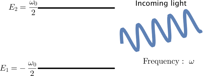
../../_images/rabi-diagram.png — Fig. 1.13 Rabi oscillation system¶

The system is prepared in low energy state. When the incoming light frequency matches the energy gap between two states, we have a resonance. Otherwise, we still have the transition from low energy state to high energy state but with a smaller transition amplitude.

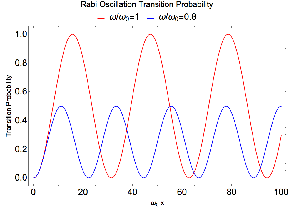
../../_images/rabi-oscillations.png — Fig. 1.14 Rabi oscillations for two differen incoming light frequencies. $ω / ω_{0} = 1$ is the resonance condition.¶

What we really mean by resonance is that the transition amplitude is maximized. Or the phase inside the off-diagonal element of Hamiltonian is minimized.

What’s more, we explore the transition amplitude as a function of differen incoming light frequencies.

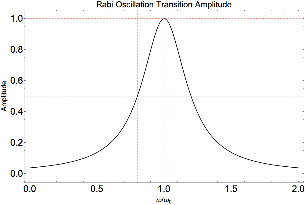
../../_images/rabi-resonance.png — Fig. 1.15 Resonance of Rabi oscillations.¶

../../_images/stimulated-probability-apmlitude-vs-k.svg — Fig. 1.16 Probabiity Amplitude as a function of $k / ω_{m}$ within RWA, with parameters $A = 0.1, θ_{m} = π / 5, ϕ = 0$ .¶

../../_images/stimulated-probability-apmlitude-vs-k-non-RWA.svg — Fig. 1.17 Probabiity Amplitude as a function of $k / ω_{m}$ for each term in Jacobi-Anger expansion, with parameters $A = 0.1, θ_{m} = π / 5, ϕ = 0$ .¶

To look at the resonances I define a Mathematica function to calculate the FWHM.

Find FWHM Using Mathematica

The Mathematica code:

fwhm[n_] := First@Differences[k /. {ToRules@Reduce[amplitude[k, 0.1, Pi/5, n] == 0.5 &&k > (1 - 0.5/Exp[n]/n^2)/n && k < (1 + 0.5/Exp[n]/n^2)/n, k]}]

../../_images/stimulated-probability-apmlitude-vs-k-resonance-width.svg — Fig. 1.18 Width of the resonances for $A = 0.1, θ_{m} = π / 5, ϕ = 0$ .¶

How do we understand the resonance? Resonance width of each order of resonance (each n) should be calculated analytically.

Lorentzian Distribution

Three-parameter Lorentzian function is

f_{x_{0}, σ, A} (x) = \frac{1}{π} \frac{σ}{σ^{2} + (x - x_{0})^{2}},

which has a width $2 γ$ .

To find the exact width is hopeless since we need to inverse Bessel functions. Nonethless, we can assume that the resonance is very narrow so that ${| F |}^{2}$ doesn’t change a lot. With the assumption, the FWHM is found be setting the amplitude to half, which is

Γ = | \frac{\hat{F}}{n_{0}} | = | \hat{k} \tan 2 θ_{m} \frac{J_{n_{0}} (n_{0} \hat{A} \cos 2 θ_{m} / \hat{k})}{n_{0}} | .

To verify this result, we compare it with the width found numerically from the exact amplitude.

Given this result, and equation (1.14), we infer that the coefficient in front of the phase term of 12 element in Hamiltonian is related to the width, while the the deviation from the exact resonance is given by $\hat{g} = n_{0} \hat{k} - 1$ .

Guessing The Width

Given a Hamiltonian 12 element here

h = \frac{F}{2} e^{i (n_{0} \hat{k} - 1) \hat{x}} = \frac{F}{2} e^{i \hat{g} \hat{x}},

the width of the resonance is

(1.17)¶

Γ = | \frac{F}{n_{0}} | .

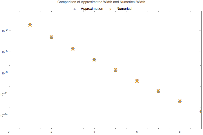
../../_images/stimulated-single-frequency-width-approximation-amp-point1.png — Fig. 1.19 Comparison of approximated width and numerical results for perturbation amplitude $\hat{A} = \frac{A}{ω_{m}} = 0.1$ .¶

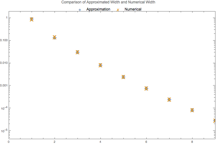
../../_images/stimulated-single-frequency-width-approximation-amp-1.png — Fig. 1.20 Comparison of approximated width and numerical results for perturbation amplitude $\hat{A} = \frac{A}{ω_{m}} = 1$ .¶

A Special Property of Bessel Function

A special relation of Bessel function is that [Ploumistakis2009]

J_{n} (n \sech α) \sim \frac{e^{n (\tanh α - α)}}{\sqrt{2 π n \tanh α}}

for large $n$ . As a matter of fact, for all positive $α$ , we always have $\tanh α - α < 0$ .

Using this relation and defining $\sech α = A \cos 2 θ_{m}$ , which renders

(1.18)¶

α = 2 n π i + \ln (\frac{1 \pm \sqrt{- A^{2} \cos^{2} 2 θ_{m} + 1}}{A \cos 2 θ_{m}}), n \in Integers,

where the Mathematica code to solve it is shown below,

In[1]:= Solve[Exp[z] + Exp[-z] == 2/(A Cos[2 Subscript[[Theta], m]]), z] // FullSimplify

we find out an more human readabale analytical expression for the width

Γ = | 2 \hat{k} \tan 2 θ_{m} \frac{e^{n (\tanh α - α)}}{n_{0} \sqrt{2 π n_{0} \tanh α}} |

where $α$ is solved out in (1.18).

For small $α$ , we have expansions for exponentials and hyperbolic functions $\tanh α \sim α - \frac{α^{3}}{3}$ ,

Γ ≍ 2 \tan 2 θ_{m} \frac{e^{n α^{3} / 3}}{\sqrt{2 π α} n_{0}^{3 / 2}} .

However, it doesn’t really help that much since $n$ is large and no expansion could be done except for significantly small $α$ .

Ploumistakis2009

Ploumistakis, S.D. Moustaizis, I. Tsohantjis, Towards laser based improved experimental schemes for multiphoton pair production from vacuum, Physics Letters A, Volume 373, Issue 32, 3 August 2009, Pages 2897-2900, ISSN 0375-9601, http://dx.doi.org/10.1016/j.physleta.2009.06.015.

(http://www.sciencedirect.com/science/article/pii/S0375960109007166) Keywords: Pair production; Multiphoton processes; High intensity lasers

1.1.4.3. Perturbation Amplitude and Transition Probability¶

../../_images/pltPertAmpPertWaveNumTransitionAmp.svg — Fig. 1.21 Transition probability amplitude at different perturbation amplitude and perturbation wavenumber.¶