1.2.6. Dispersion Relation and Crossing¶

How to understand Dispersion Relation

We should come back to the wave picture. DR tells us how easily a wave will disperse as it travels. The things that can be research on are the disperse itself. Stability is one important topic but it also tells us how the wave disperse.

1.2.6.1. Box Spectrum¶

Box Spectrum Defined Spectra Code

spectWC1 = {{{-1, -0.3}, 1}, {{-0.3, 1}, 1}};
spectWC2 = {{{-1, -0.3}, 0.5}, {{-0.3, 1}, 1}};
spectWC3 = {{{-1, -0.3}, 0.1}, {{-0.3, 1}, 1}};
spectWC4 = {{{-1, -0.3}, 0}, {{-0.3, 1}, 1}};

spectC1 = {{{-1, -0.3}, -0.1}, {{-0.3, 1}, 1}};
spectC2 = {{{-1, -0.3}, -0.5}, {{-0.3, 1}, 1}};
spectC3 = {{{-1, -0.3}, -1}, {{-0.3, 1}, 1}};
spectC4 = {{{-1, -0.3}, -1.5}, {{-0.3, 1}, 1}};

spectC5 = {{{-1, -0.3}, -15}, {{-0.3, 1}, 1}};
spectC6 = {{{-1, -0.3}, -0.01}, {{-0.3, 1}, 1}};
spectC7 = {{{-1, -0.3}, 0.01}, {{-0.3, 1}, 1}};
spectWC5 = {{{0.1, 0.3}, 1}, {{0.3, 1}, 1}};

Numerical Issues with Box Spectrum in LSA

Mathematica seems to fail the mission when finding the complex k’s given real \(\omega\).

I tested bot NIntegrate of the integrals and Integrate first. It seems that Integrate first works better and faster.

Since I could find the analytical expressions for the integrals, I simple plug in the expression then calculate numbers.

I could plot the values of \(\omega - (I_0-I_4)/4\) (MAA solution) for real \(\omega\) to check if they have interceptions with the 0 plane.

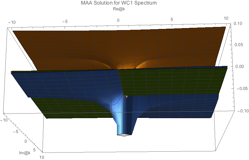
../../_images/maa-solution-real-image-3d-plot-spect-wc1.png — Fig. 1.134 MAA solution for WC1 spectrum. This plot was for \(\omega=0.1\). The two horizontal axes are real and imaginary part of k. Green plane is 0 plane. The blue surface is real part while the orange surface is imaginary part. We could see the spike-like structure in the real part intercepts with 0 plane as well as imaginary part that indicates a solution¶

I also ploted out the MZA solutions. I found that interceptions exsits for only some values of \(\omega\). Examples of such plots are shown below.

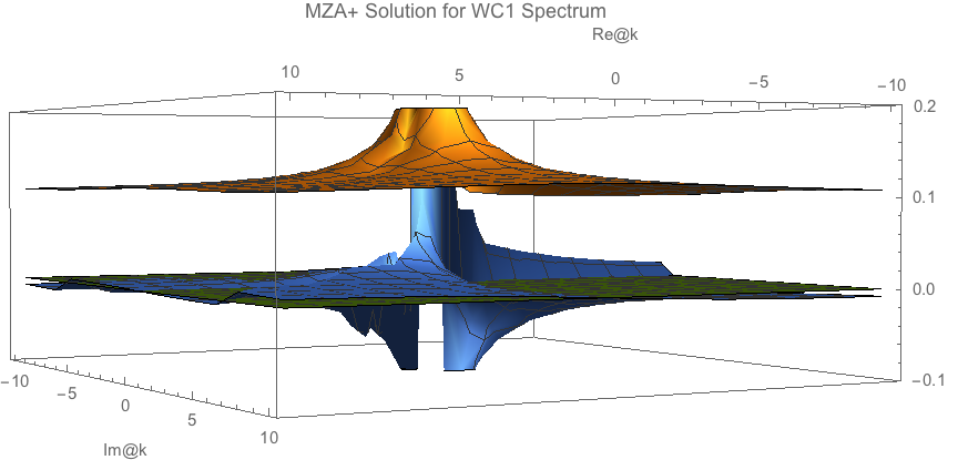
../../_images/mzap-solution-real-image-3d-plot-spect-wc1.png — Fig. 1.135 MZA+ solutions for spectrum id WC1. Seems to be solutionless.¶

Similarly for MZA- solution we have the following.

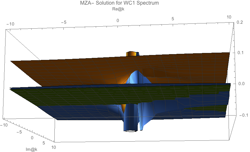
../../_images/mzam-solution-real-image-3d-plot-spect-wc1.png — Fig. 1.136 MZA- solutions for spectrum id WC1.¶

After some test, my thought is that the integral is nicely behaved for some range of real \(\omega\), which makes sense since the line of instability can not extend to arbitary large and small \(\omega\).

Thus the solution to the warnings and errors in FindRoot is to plugin the suitable range of \(\omega\).

Meanwhile for real \(k\), we have only solutions at \(\omega =0\).

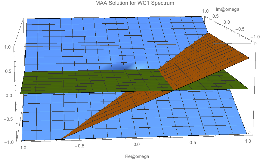
../../_images/maa-solution-real-image-3d-plot-spect-wc1-realk.png — Fig. 1.137 For real k. MAA solution. Blue, Orange, Green has similar means as before.¶

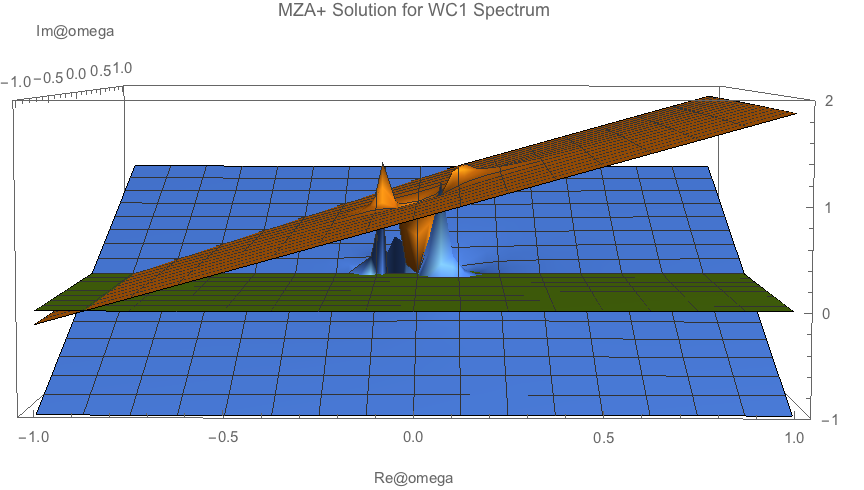
../../_images/mzap-solution-real-image-3d-plot-spect-wc1-realk.png — Fig. 1.138 For real k, \(k=0.1\).¶

MAA solutions also has similar shape.

In any case, we managed to solve instabilities for MAA and MZA. In Mathematica package dispersion-relation.wl, ConAxialSymOmegaNMZApEqnLHSComplex[-omegareal, k, spectrum] returns the value of \(\omega - \left( -\frac{1}{4}\left( I_0 - I_2 + \sqrt{ (I_0+I_2-2I_1)(I_0+I_2+2I_1) } \right) \right)\). Simply using FindRoot from Mathematica should return the solutions.

Since box spectrum is easier and faster to calculate, we’ll explore the phenomena within box spectrum. For example, the spectrum notation

{{{-1, -0.3}, -0.2}, {{-0.3, 1}, 0.7}}

indicates tht the spectrum has a constant value -0.2 within \(\cos\theta \in [-1,-0.3]\) and value 0.7 within \(\cos\theta \in [-0.3,1]\).

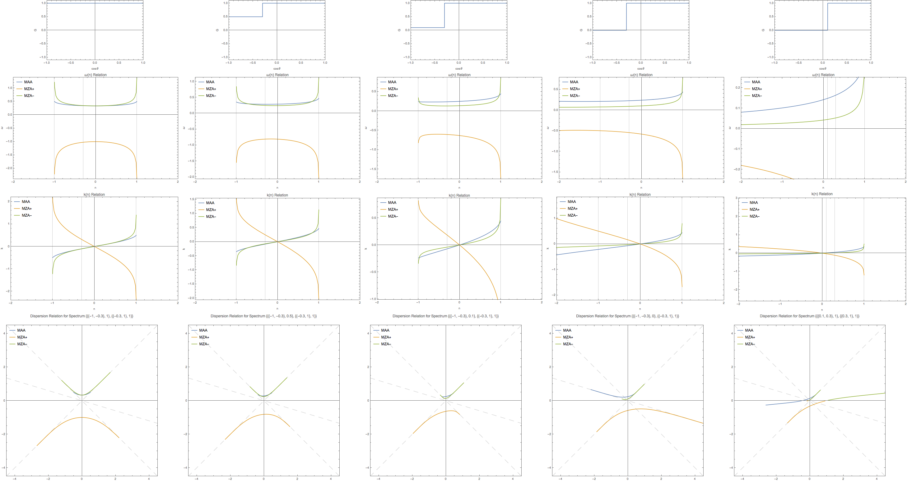
../../_images/box-spectra-without-crossing-omega-n-k-n-dr.png — Fig. 1.139 No crossing¶

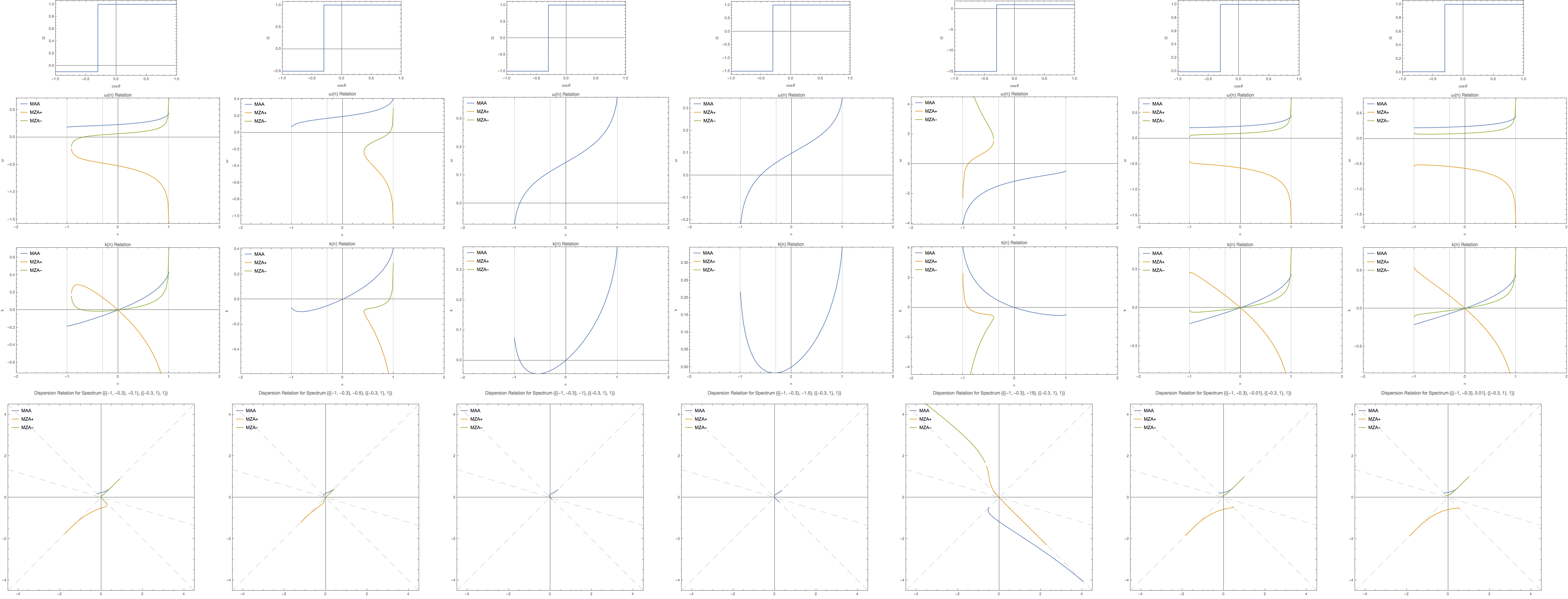
../../_images/box-spectra-with-crossing-omega-n-k-n-dr.png — Fig. 1.140 With crossing¶

Observations and Questions

Any 0 in spectrum make it possible go cross the singularity line.
MZA disappears at some point of parameters. What are the constraints.

MZA disappears

The analytical expression for it to dispear shows that it involves all the elements of the spectrum. Numerically, I can show that for a specific one \(\{\{\{-1, -0.3\}, g_1\}, \{\{-0.3, 1\}, 1\}\}\), the region of \(g_1\) that leads to no MZA solution for a given \(n\) is shown in Fig. 1.141.

../../_images/analytical-where-mza-dispear-spectrum-c5.png — Fig. 1.141 Region of \(g_1\).¶

This figure shows that the MZA solution will come back if we choose really small \(g_1\). It is verified using another spectrum which is labeled as C5 spectrum.

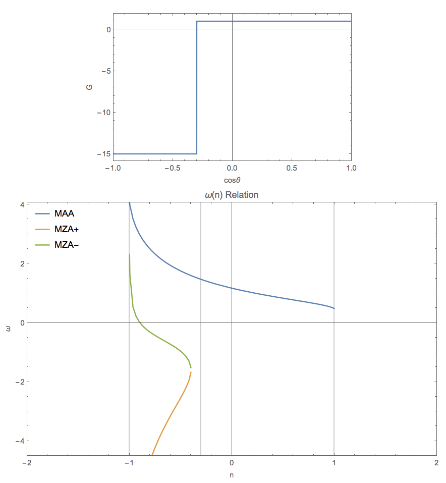
../../_images/omega-n-spectrum-c5.png — Fig. 1.142 For a spectrum \(\{\{\{-1, -0.3\}, -15\}, \{\{-0.3, 1\}, 1\}\}\).¶

However examples of numerical calculations won’t be enough. Alternatively, I could derive an analytical expression. MZA solution is

\[\omega = -\frac{1}{4}\left(I_0-I_2\pm \sqrt{ (I_0-2I_1+I_2)(I_0+2I_1+I_2) }\right).\]

We examine the term inside square root and set it to be negative which will show us the region where real omega disppears.

Comment: the upper limit is not a horizontal line.

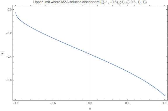
../../_images/omega-n-upper-limit-spectrum-c5.png — Fig. 1.143 Upper limit.¶

For the MZA solutions to disappear, we need to find the smallest value of the upper limit (-0.73160 in this case) and the largest value of lower limit (-7.16327 in this case).

Taylor Expansion of MZA solutions

What about Taylor expansion around small values of \(g_1\)? Taylor expanding the most general abstract form doesn’t give us any useful results since it is super complicated.

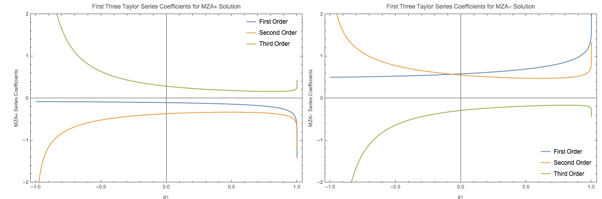
../../_images/mza-solutions-taylor-series-coefficients-spect-c5.png — Fig. 1.144 Coefficients of Taylor series of MZA solutions. It’s weird that the coefficients are all real.¶

I am not sure how to use these results.

Crossing has an effect on \(d\omega/dn\)

By observing the \(\omega\sim n\) plot, we noticed that crossing is changes the behavior of it, especially at the point \(n=-1\). It seems that crossing changes whether the \(\omega\) goes to \(\infty\) or \(-\infty\) at \(n=-1\).

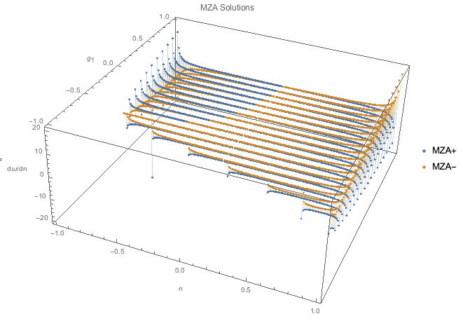
../../_images/box-spectra-mza-g1-n-shortrange.png — Fig. 1.145 \(d\omega/dn\) for MZA solutions with spectrum \(spectAbs2 = \{\{\{-1, -0.3\}, g_1\}, \{\{-0.3, 1\}, 1\}\}\). In this plot, we have \(g_1\in [-1,1]\) with a step size 0.1 while \(n\in [-1,1]\). We notice that the value at -1 changes as crossing happens.¶

More specifically, we plot out the \(d\omega/dn\) for three different \(g_1\).

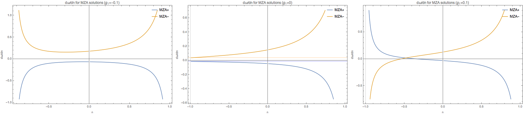
../../_images/box-spectra-mza-n-g1-three-values-including-crossing.png — Fig. 1.146 for 3 different values of \(g_1\). The second panel is for \(g_1=0\). The grid lines are actually calculated using Limit which are \(-0.0143723\) and \(0.0370502\). They never become 0?¶

MZA solutions Disapears?

The DR plots show that MZA solutions disappears for spectC3 and spectC4. Is this true?

I tested Exclusions->None in Mathematica to make sure this is not a plotting issue. The results do not change with this option.

However, I found that the \(\lvert f(\omega=1,k)\rvert\) is approaching 0 for some none zero real k.

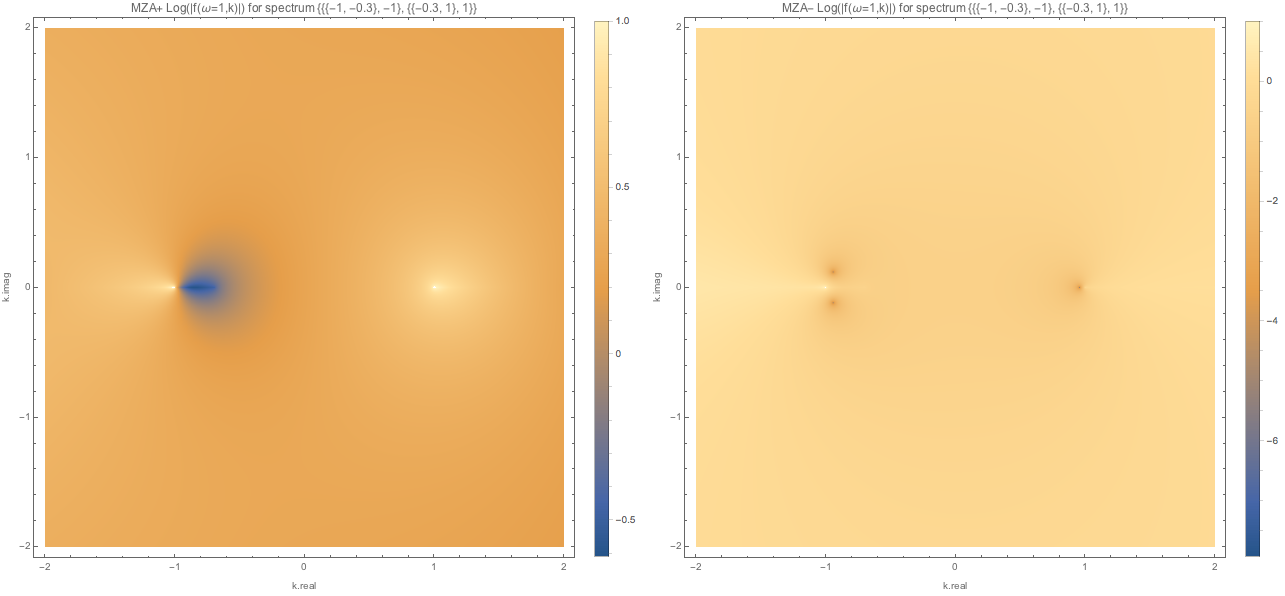
../../_images/f-of-omega-1-and-k-densityplot-log-mzap-mzam-spectc3.png — Fig. 1.147 MZA solutions for `spectC3` with \(\omega=1\). We found one real solutioin for MZA- solution, which is not what we expected from DR plots.¶

This makes the DR plots questionable. However, no bug has been found. In fact I have been using the same functions to make this density plot.

The I realized that using only real \(n\)’s could be a problem since we might have complex \(n\)’s that give us real \(\omega\), in principle.

Indeed this is true for spectC3.

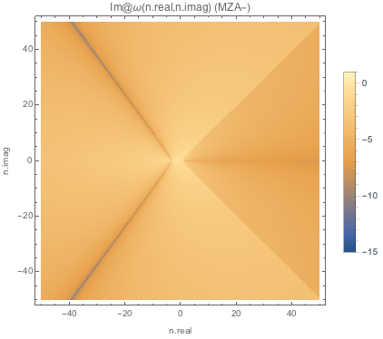
../../_images/imaginary-part-of-omega-for-complex-n-mzap-boxspectrum-spectc3.png — Fig. 1.148 Absolute value of imaginary part of \(\omega\) for MZA+ solution of `spectC3`¶

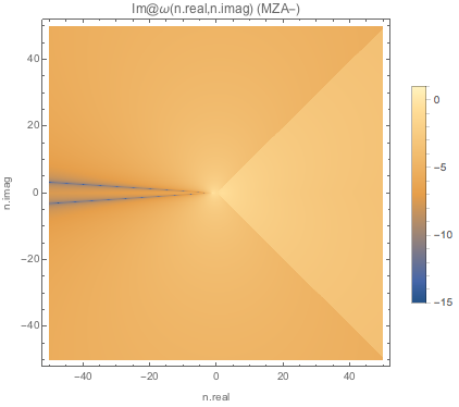
../../_images/imaginary-part-of-omega-for-complex-n-mzam-boxspectrum-spectc3.png — Fig. 1.149 Absolute value of imaginary part of \(\omega\) for MZA- solution of `spectC3`.¶

Meanwhile the real parts of these solutions do not go to 0.

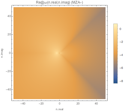
../../_images/real-part-of-omega-for-complex-n-mzap-boxspectrum-spectc3.png — Fig. 1.150 Absolute value of real part of \(\omega\) for MZA+ solution of `spectC3`.¶

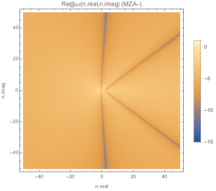
../../_images/real-part-of-omega-for-complex-n-mzam-boxspectrum-spectc3.png — Fig. 1.151 Absolute value of real part of \(\omega\) for MZA- solution of `spectC3`.¶

But there can never be real k for these real \(\omega\) lines because real \(k=\omega n\) where \(n\) is complex.

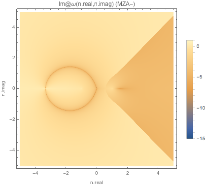
../../_images/imaginary-part-of-k-for-complex-n-mzap-boxspectrum-spectc3.png — Fig. 1.152 Absolute value of imaginary part of \(k\) for MZA+ solution of `spectC3`.¶

For spectC3, we have the following.

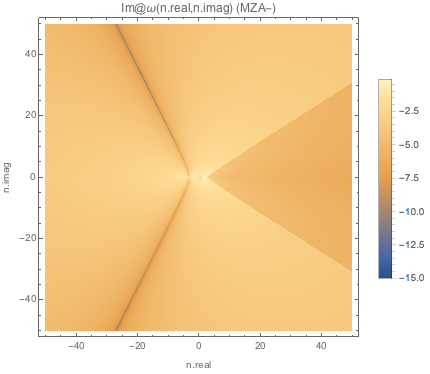
../../_images/imaginary-part-of-omega-for-complex-n-mzap-boxspectrum-spectc2.png — Fig. 1.153 Absolute value of imaginary part of \(\omega\) for MZA+ solution of `spectC2`.¶

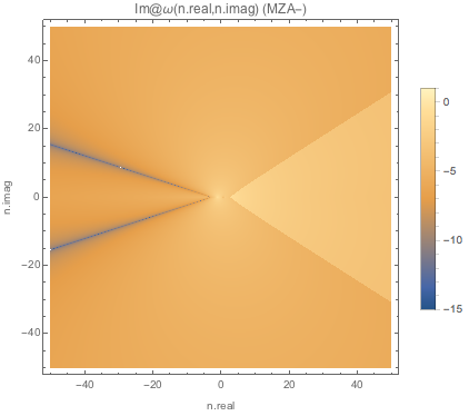
../../_images/imaginary-part-of-omega-for-complex-n-mzam-boxspectrum-spectc2.png — Fig. 1.154 Absolute value of imaginary part of \(\omega\) for MZA- solution of `spectC2`.¶

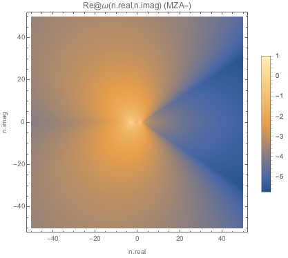
../../_images/real-part-of-omega-for-complex-n-mzap-boxspectrum-spectc2.png — Fig. 1.155 Absolute value of real part of \(\omega\) for MZA+ solution of `spectC2`.¶

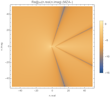
../../_images/real-part-of-omega-for-complex-n-mzam-boxspectrum-spectc2.png — Fig. 1.156 Absolute value of real part of \(\omega\) for MZA- solution of `spectC2`.¶

So things must be special for spectWC1 etc. Here we plot the real and imaginary part of spectWC3.

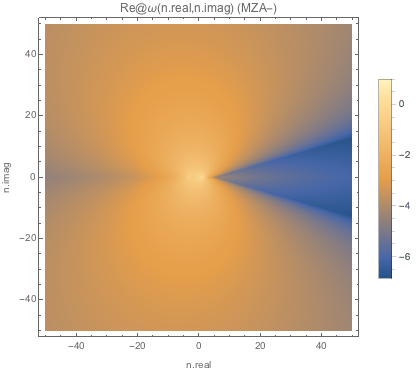
../../_images/real-part-of-omega-for-complex-n-mzap-boxspectrum-spectwc3.png — Fig. 1.157 Absolute value of real part of \(\omega\) for MZA+ solution of `spectWC3`.¶

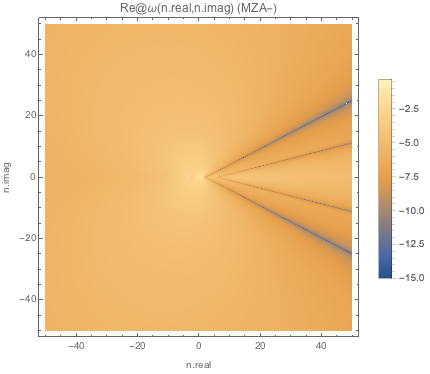
../../_images/real-part-of-omega-for-complex-n-mzam-boxspectrum-spectwc3.png — Fig. 1.158 Absolute value of real part of \(\omega\) for MZA- solution of `spectWC3`.¶

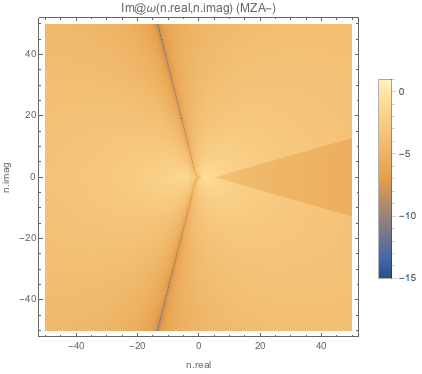
../../_images/imaginary-part-of-omega-for-complex-n-mzap-boxspectrum-spectwc3.png — Fig. 1.159 Absolute value of imaginary part of \(\omega\) for MZA+ solution of `spectWC3`.¶

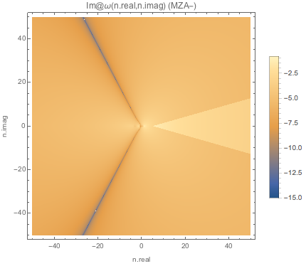
../../_images/imaginary-part-of-omega-for-complex-n-mzam-boxspectrum-spectwc3.png — Fig. 1.160 Absolute value of imaginary part of \(\omega\) for MZA- solution of `spectWC3`.¶

But there can never be real k for these real \(\omega\) lines because real \(k=\omega n\) where \(n\) is complex.

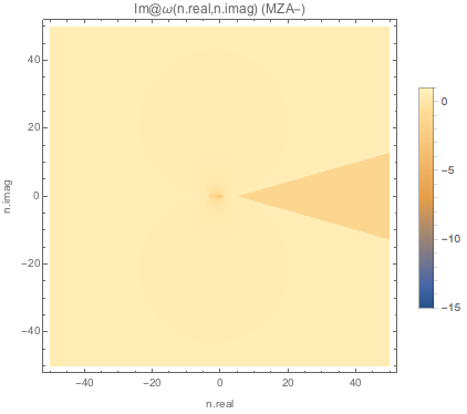
../../_images/imaginary-part-of-k-for-complex-n-mzap-boxspectrum-spectwc3.png — Fig. 1.161 Absolute value of imaginary part of \(k\) for MZA+ solution of `spectWC3`.¶

So, where did the MZA solutions go?

1.2.6.1.1. Instabilities for Box Spectra¶

Crossing seems to have little effects on instabilities

Instabilities on DR plot seems to be NOT affected by crossing. Probably because of the lines in the forbidden region (using abs for log argument in the results of integral for I’s) doesn’t seem to change a lot.

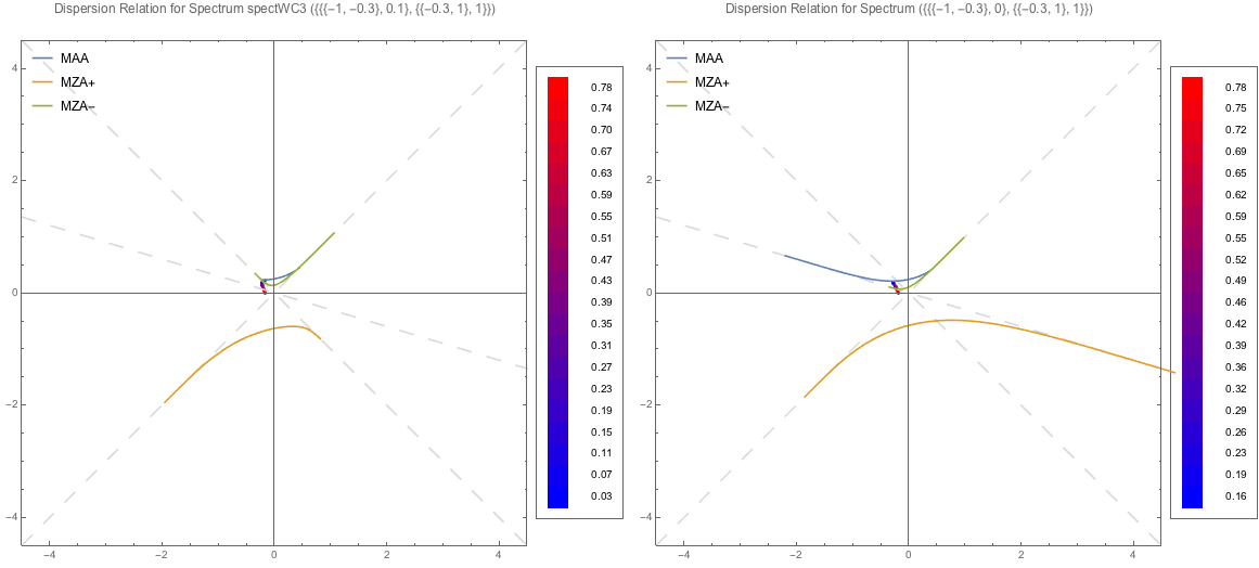
../../_images/box-spectra-dr-lsa-maa-spectwc3-to-wc4.png — Fig. 1.162 MAA DR and LSA for spectrum `spectWC3` and `spectWC4`. LSA is for real \(\omega\), the color of the dots indicates the value of imaginary value of \(k\).¶

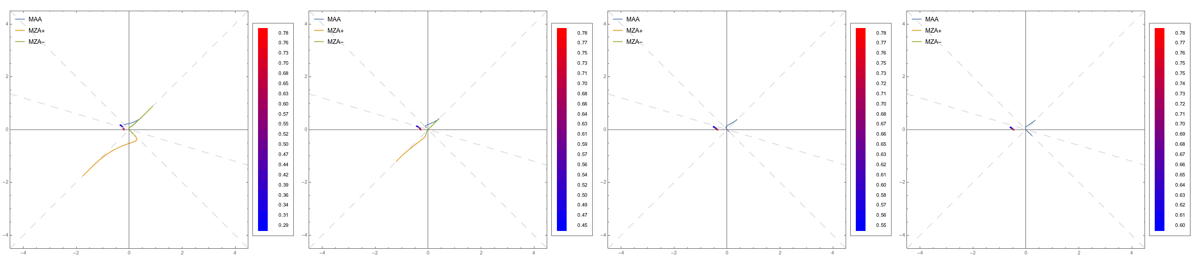
../../_images/box-spectra-dr-lsa-maa-spectc1-to-c4.png — Fig. 1.163 DR and LSA (MAA) for spectra with crossings.¶

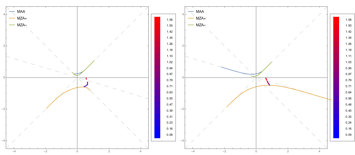
../../_images/box-spectra-dr-lsa-mzap-spectwc3-wc4.png — Fig. 1.164 DR and LSA (MZA+) for spectra `spectWC3` (left) and `spectWC4` (right).¶

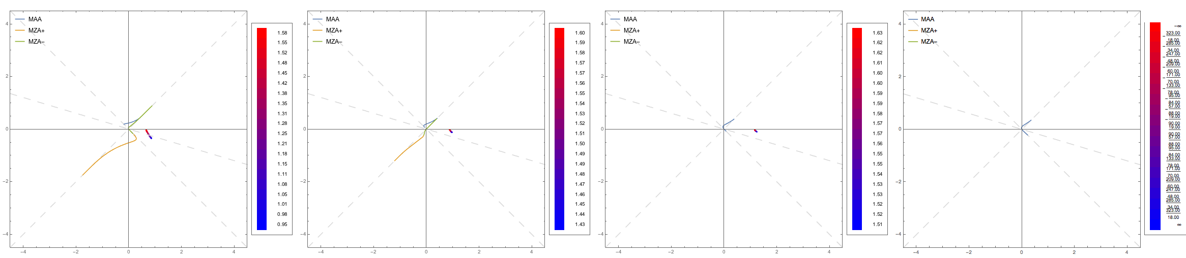
../../_images/box-spectra-dr-lsa-mzap-spectc1-to-c4.png — Fig. 1.165 DR and LSA (MZA+) for spectra `spectC1` (left-most) to `spectC4` (right-most).¶

1.2.6.2. Can We Explain Crossing Using Discrete Beams?¶

What does backward emission mean? Is it somewhat equivalent to crossing spectrum without backward emission?

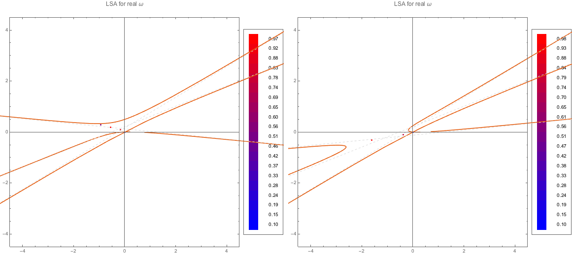
../../_images/lsaMAAROPltDB-WC4-and-C4.png — Fig. 1.166 DR and LSA (MAA) for `spectDBWC4` and `spectDBC4` which are `{{0.5, -0.1}, {1, 0.4}, {1, 0.6}}` and `{{-0.5, 0.1}, {1, 0.4}, {1, 0.6}}` respectively.¶

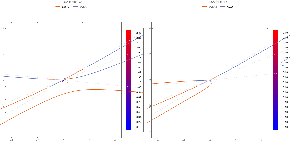
../../_images/lsaMZApROPltDB-WC4-and-C4.png — Fig. 1.167 DR and LSA (MZA+) for `spectDBWC4` and `spectDBC4` which are `{{0.5, -0.1}, {1, 0.4}, {1, 0.6}}` and `{{-0.5, 0.1}, {1, 0.4}, {1, 0.6}}` respectively.¶

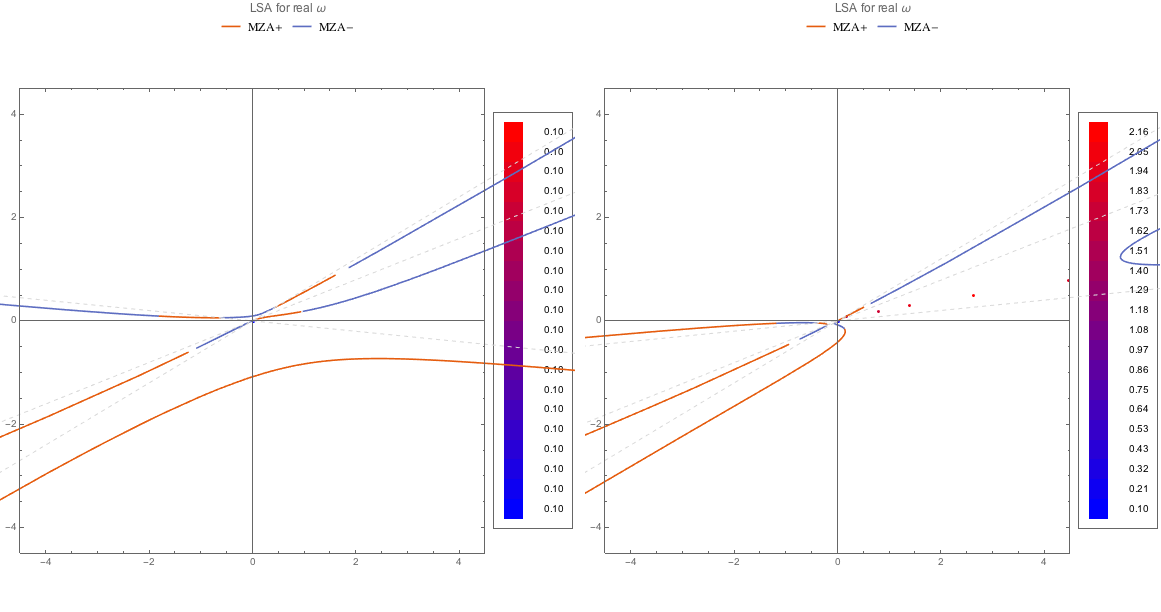
../../_images/lsaMZAmROPltDB-WC4-and-C4.png — Fig. 1.168 DR and LSA (MZA-) for `spectDBWC4` and `spectDBC4` which are `{{0.5, -0.1}, {1, 0.4}, {1, 0.6}}` and `{{-0.5, 0.1}, {1, 0.4}, {1, 0.6}}` respectively.¶

Analytically, crossing and backward emission are not simply related.

1.2.6.3. Spectral Crossing Makes DR Crossing 0 Possible¶

The MZA solution has some interesting behaviors. It seems that a crossing in spectrum can bend the DR and make it cross 0.

We can prove that the crossing indeed needed but not guarantee to make DR cross 0.

The MZA solution is

\[(-4\omega -(I_0 - I_2) )^2 = (I_0 -2 I_1 + I_2)(I_0 + 2 I_1 + I_2).\]

For \(\omega\to 0\), we have

\[I_0I_2 = I_1^2.\]

We restore the integral form, which is

\[\int du \frac{ G(u) u^2 }{ 1- n u} = \left( \int du \frac{ G(u) u }{ 1- n u} \right)^2.\]

We actually have \(1-n u>0\). Thus

\[\tilde G (u) = \frac{G(u)}{1-n u},\]

always preserves the sign of the spectrum. If the spectrum is always positive, then we are calculating some average of \(u\) and \(u^2\), the equation becomes

\[\langle u^2 \rangle = \left(\langle u \rangle \right)^2,\]

which can not be true. However, a crossing brings some negative regions and makes it possible but not guaranteed to have solutions.