1.2.5. Dispersion Relation and Gap
1.2.5.1. Discrete Beams
I define the following beams,
spectDBWC1 = {{1, -0.6}, {1, 0.1}, {1, 0.6}}
spectDBWC2 = {{0.5, -0.6}, {1, 0.1}, {1, 0.6}}
spectDBWC3 = {{0.1, -0.6}, {1, 0.1}, {1, 0.6}}

spectDBC1 = {{-1, -0.6}, {1, 0.1}, {1, 0.6}}
spectDBC2 = {{-0.5, -0.6}, {1, 0.1}, {1, 0.6}}
spectDBC3 = {{-0.1, -0.6}, {1, 0.1}, {1, 0.6}}
The first thing is to really see that the instability regions are going through the gap in discrete beams case.
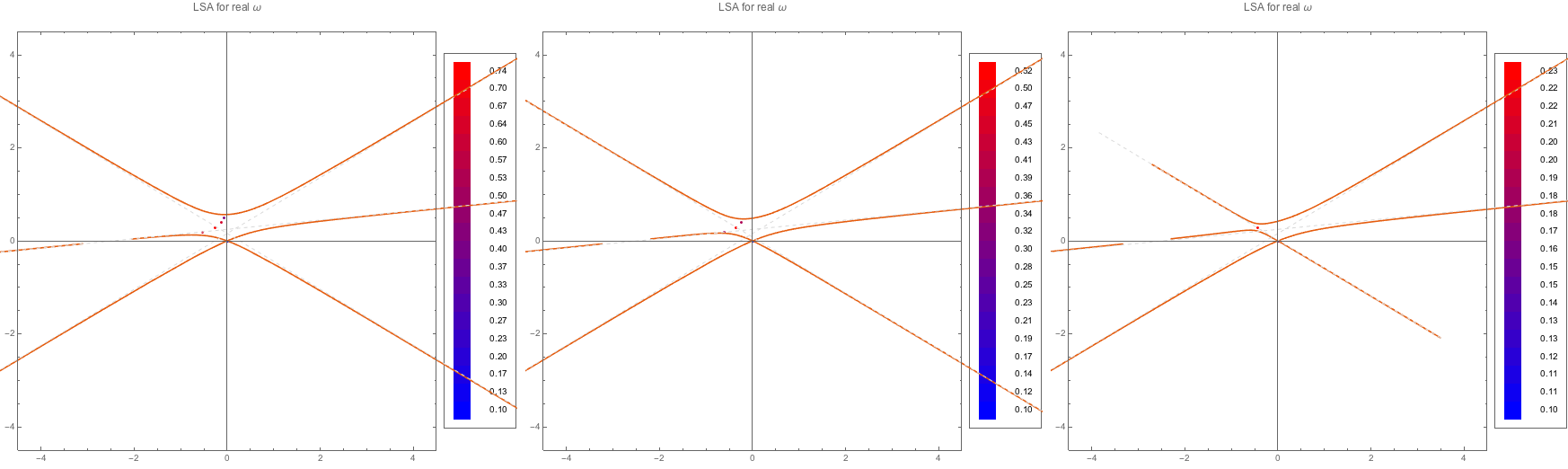
Fig. 1.100 MAA solutions for spectra WC1, WC2, WC3. The instability regions go through the gap.

Fig. 1.101 MAA solutions for spectra C1, C2, C3. For real \(\omega\), no complex k is found.
The MZA+ solution can also be found.
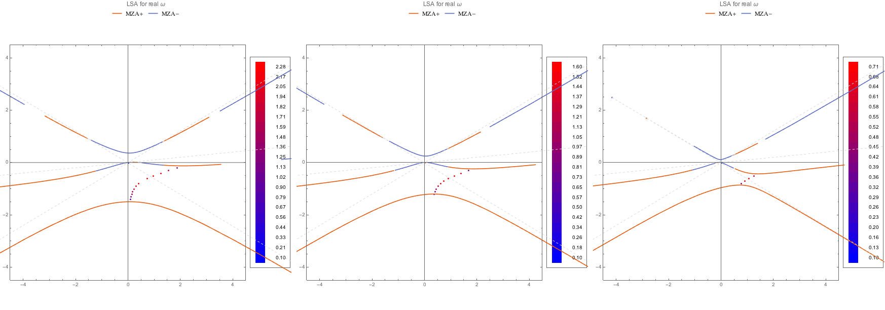
Fig. 1.102 MZA+ solution for WC spectra.
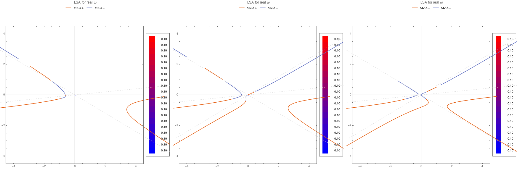
Fig. 1.103 MZA+ solution for C spectra. As like before, no instability in k is found.
The MZA- solutions:
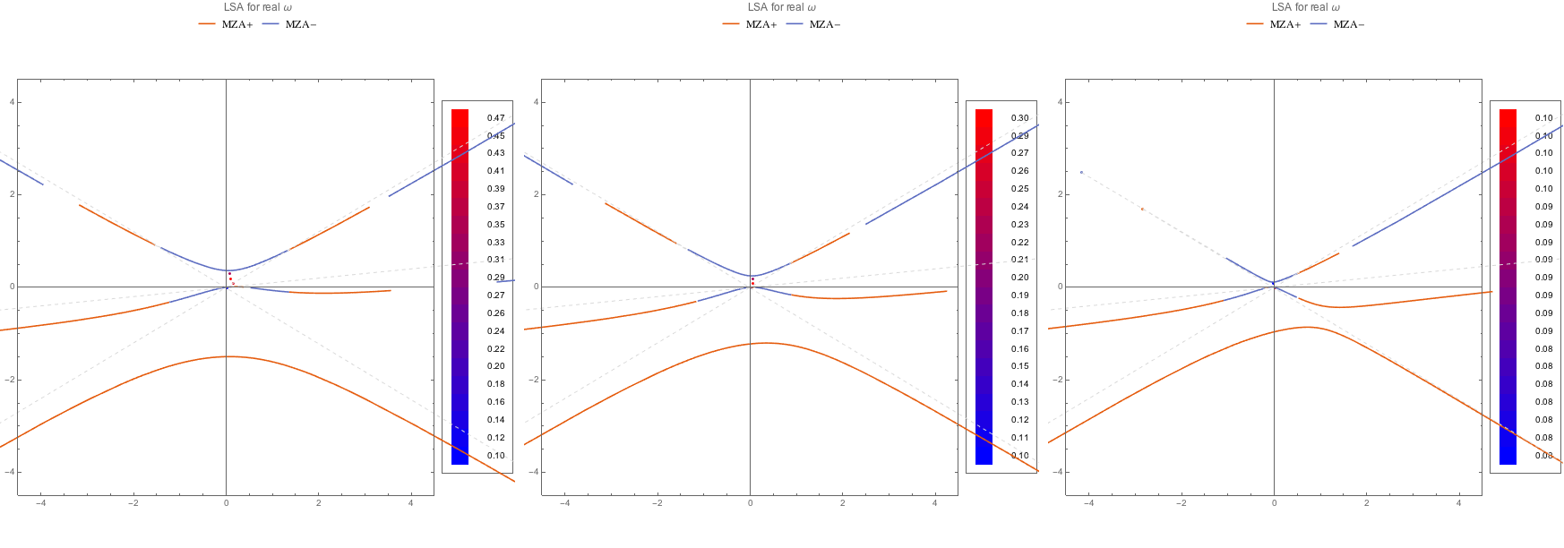
Fig. 1.104 MZA- solution for WC spectra.

Fig. 1.105 MZA- solution for C spectra.
So the C spectra have no instabilities in k. I should calculate the instabilities in \(\omega\) for real k.
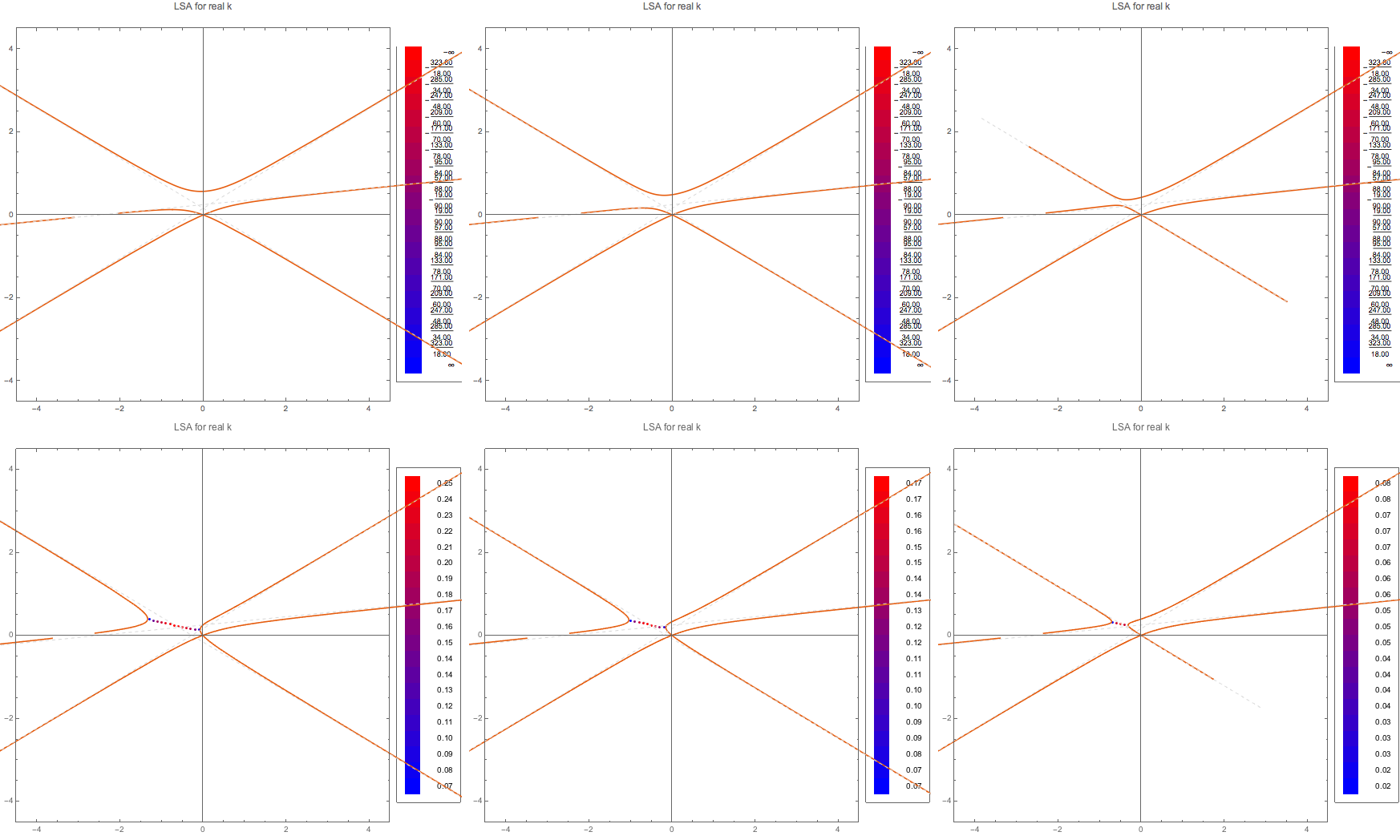
Fig. 1.106 MAA solution for real k finding complex \(\omega\).
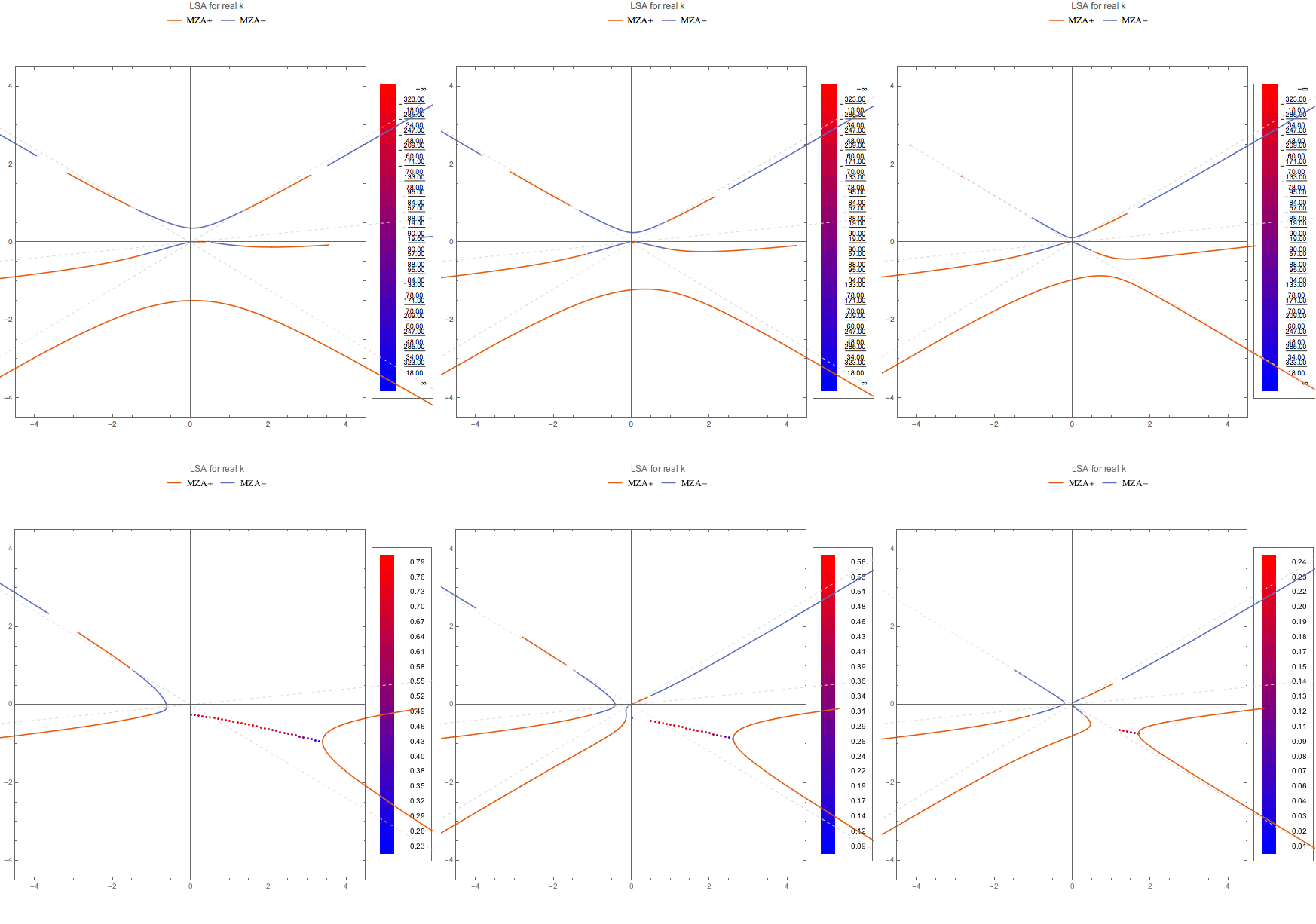
Fig. 1.107 MZA+ solution for real k finding complex \(\omega\).
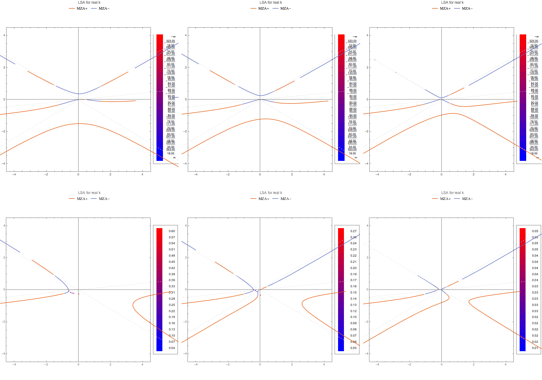
Fig. 1.108 MZA- solution for real k finding complex \(\omega\).
1.2.5.2. Two Beams
For two beams, the equation \(f(\omega,k)=0\) is quadratic in both \(\omega\) and \(k\), thus two solutions everywhere even for complex solutions.
Infinities at Emission Angle
It has been a very weird thing that the MZA DR lines can cross the forbidden lines defined by the emission angle. To illustrate this problem, we think of a two beams model, with spectrum \(\{\{g_1,u_1\},\{g_2,u_2\}\}\).
The equation for DR has terms of the form
which indicates that this can lead to infinity when \(n=1/u_i\), unless the numerator is 0. For MAA solution, the numerator indeed becomes 0. But for MZA solution it is not that obvious.
However, we can prove that one of the MZA solutions is still finite as \(n=1/u_i\).
The MZA solution is
where
We are interested in wether the term
will become finite at \(n=1/u_i\). We plug in the expressions for \(I_m\).
We take the limit \(n\to 1/u_i\).
One of the solutions, + or -, will be 0, depending on spectrum and also which side we are approaching the limit.
Suppose we have \(g_1>0\) and \(n\to 1/u_1 +\) (\(1-n u_1<0\)).
so that the MZA+ solution is 0.
1.2.5.3. Solutions
It seems that gap and instability are not really related all the time. For discrete beams, the number of solutions is the key to instabilities.
It shows that spectrum \(DBC1\) has only MZA+ instabilities on the left side of the axis for real k. We need to prove that no solutions are found on the left side of the axis. Similarly for MZA- solutions but on different sides.
1.2.5.3.1. Discrete Beams
1.2.5.3.1.1. MAA
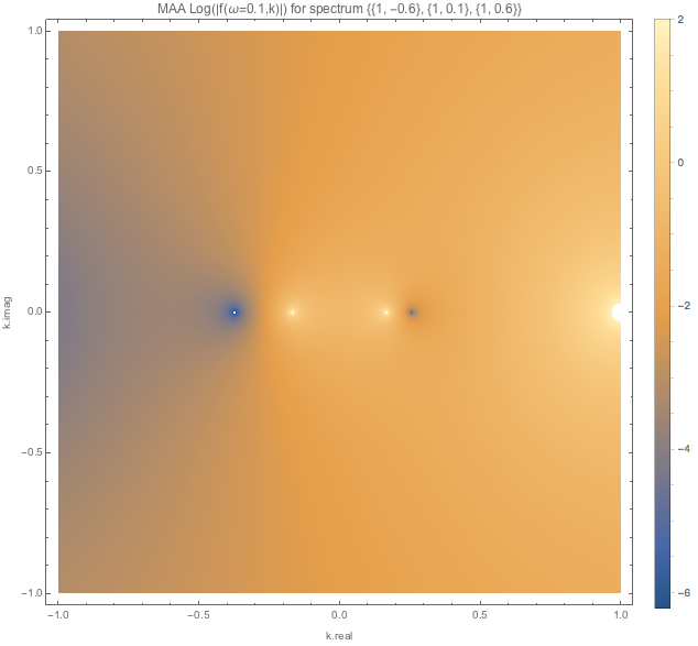
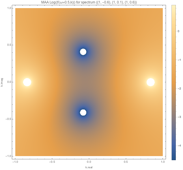
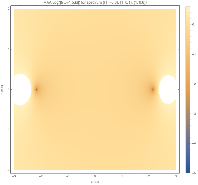
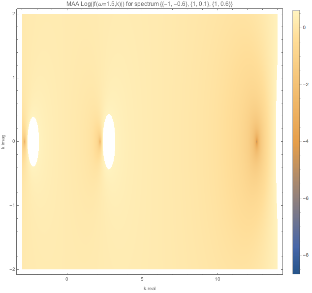
For spectDBWC1 we have the following density plots of \(f(\omega=0.1,k)\), \(f(\omega=0.5,k)\), and \(f(\omega=1.5,k)\) respectively.
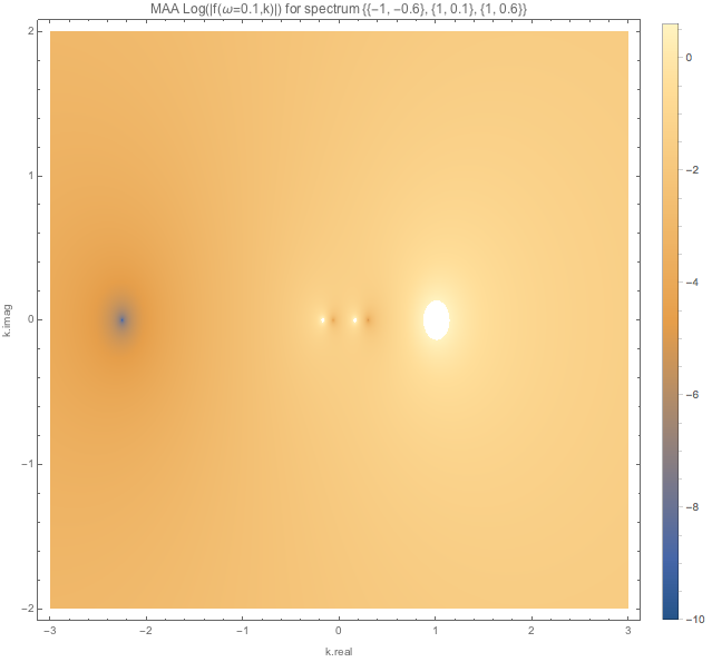
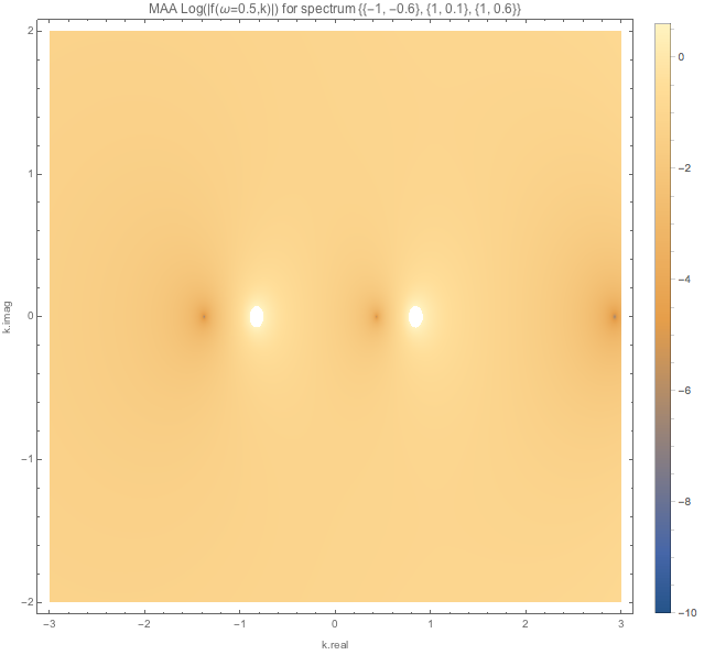
Similar plots are made for spectDBC1 which has no MAA instabilities.
1.2.5.3.1.2. MZA
I can also plot out the MZA solutions.
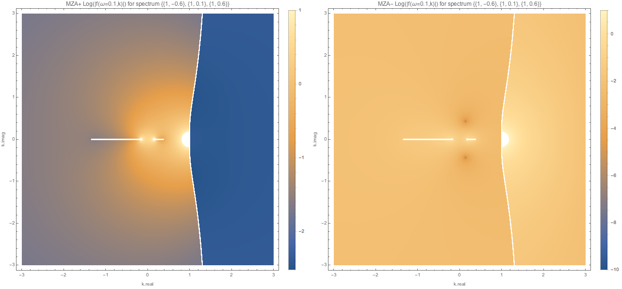
Fig. 1.109 MZA solutions (MZA+ left, MZA- right) for spectDBWC1 with \(\omega=0.1\). The MZA+ plot on the left seems to be weird. I checked the values within this region. There is a plateau here but not exactly flat. And they are not approaching 0. The other real solution in MZA- solution which is not shown is pretty far away from these two complex solutions.
A closer look at the MZA- solutions are showed below.
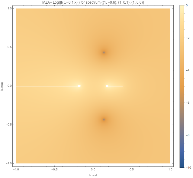
Fig. 1.110 MZA- solutions for spectDBWC1 at a closer look at the 0 points. The white bands are regions slightly larger than 0. Log@Abs@DBAxialSymOmegaNMZApEqnLHSComplex[0.1, -0.1826 - 0*I, spectDBWC1] returns 0.475377.
Check Values at Plateau
In[162]:= Log@Abs@DBAxialSymOmegaNMZApEqnLHSComplex[0.1, 1.6 - 1*I, spectDBWC1]
Log@Abs@DBAxialSymOmegaNMZApEqnLHSComplex[0.1, 1.2 - 1*I, spectDBWC1]

Out[162]= -2.46077
Out[163]= -2.49663
A sharp transition occurs at the white boundry. The values near the boundary change abruptly. According to the values \(f(\omega=0.1,k)\), imaginary part of it appears and becomes large as we move from left to right around the boundary.
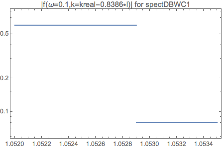
Fig. 1.111 LogPlot of \(|f(\omega=0.1,k=kreal-0.8386*I)|\) for \(kreal\in [1.052, 1.0535]\). This region of plot goes across the step structure.
LogPlot[Abs@DBAxialSymOmegaNMZApEqnLHSComplex[0.1, kreal - 0.8386*I, spectDBWC1], {kreal, 1.052, 1.0535}, Frame -> True, PlotLabel -> "|f(\[Omega]=0.1,k=kreal-0.8386*I)| for spectDBWC1"]
For \(\omega=-0.5\).
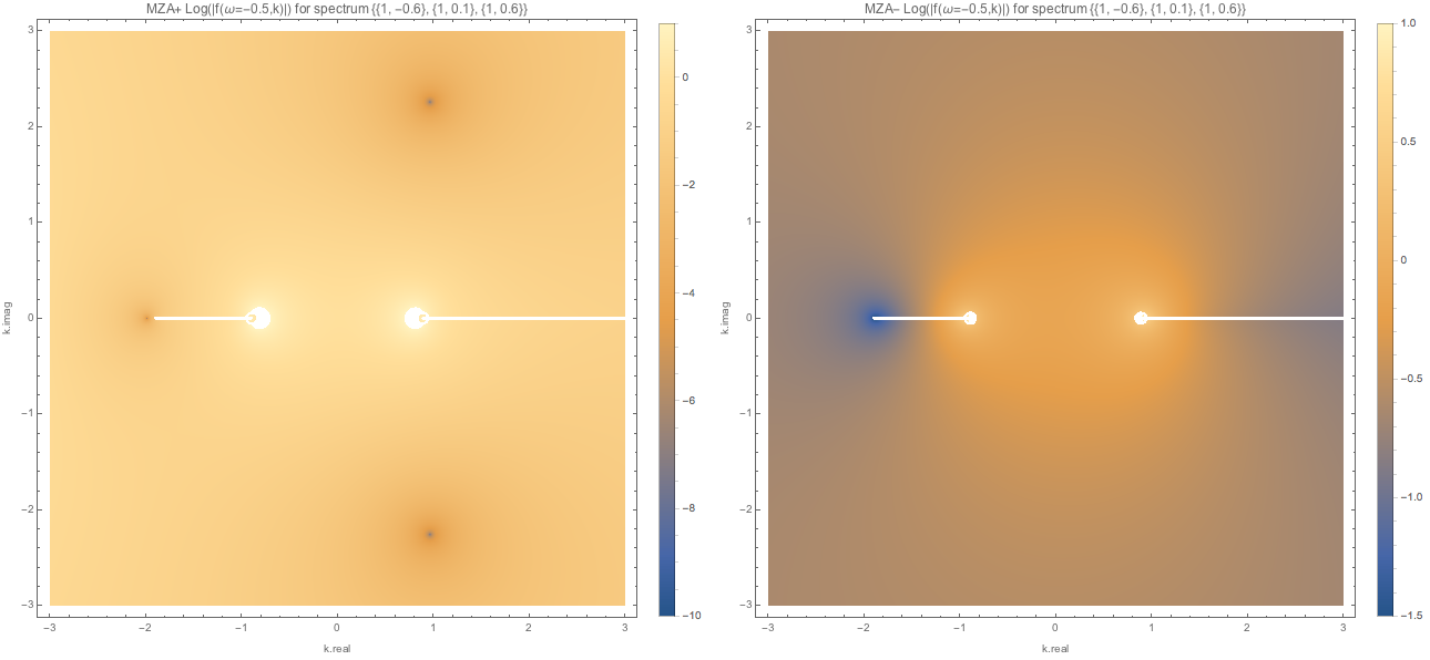
Fig. 1.112 MZA solutions (MZA+ left, MZA- right) for spectDBWC1 with \(\omega=-0.5\).
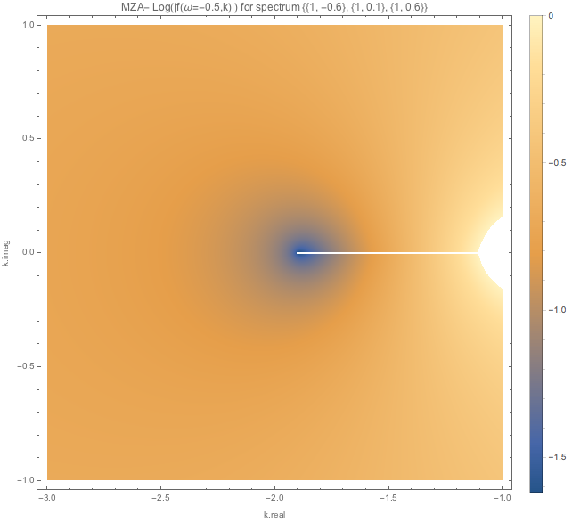
Fig. 1.113 MZA- solution around the real solution. Log@Abs@DBAxialSymOmegaNMZApEqnLHSComplex[-0.5, -1.99 - 0*I, spectDBWC1] returns -5.18447 which indicates a 0 point.
1.2.5.3.2. Box Spectra
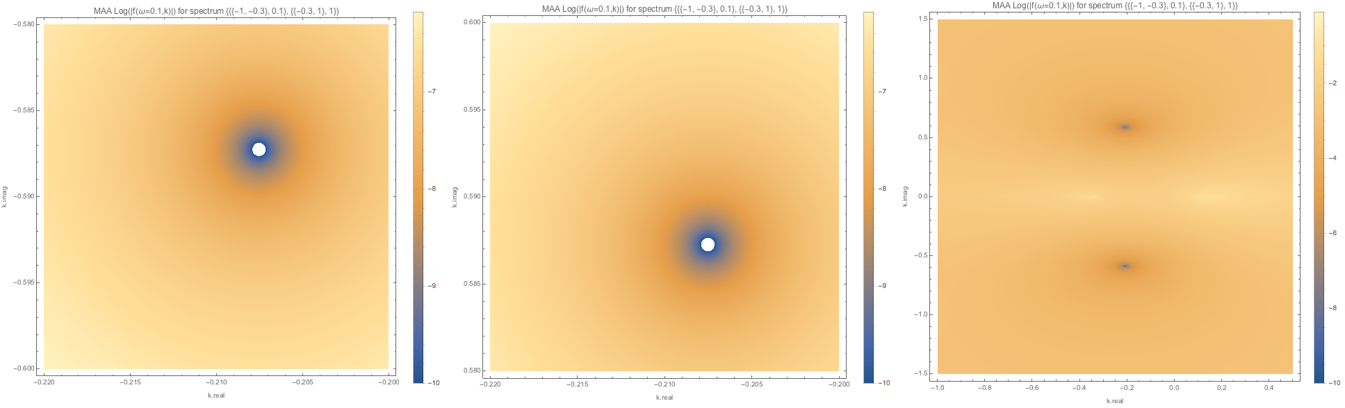
Fig. 1.114 MAA spectWC3 for \(\omega=0.1\). We have points or regions approaching \(f(\omega=0.1,k)\to 0\).
f-of-omega-m0.1-and-k-densityplot-log-maa-spectwc3.png
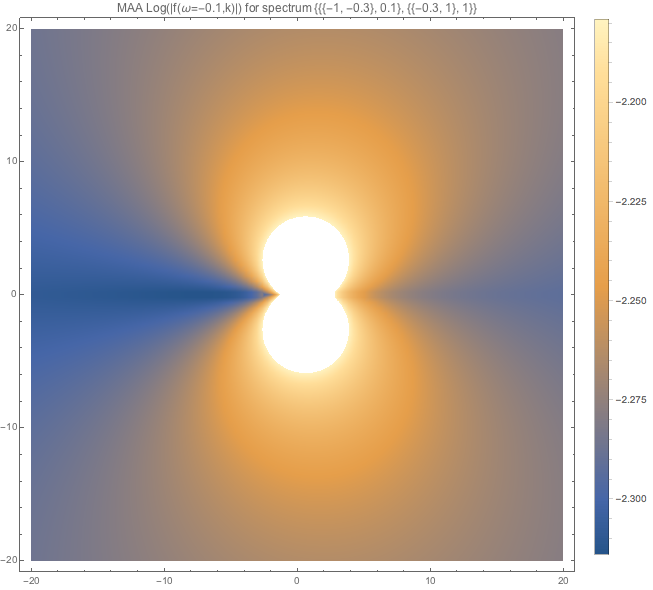
Fig. 1.115 MAA spectWC3 for \(\omega=-0.1\). How do I determine whether it is approaching 0? I change the plot range and checked. \(e^{-2.3}\) seems to be the smallest value.
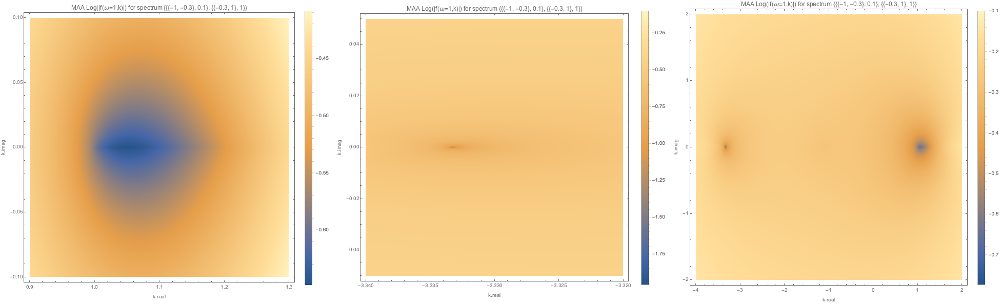
Fig. 1.116 MAA spectWC3 for \(\omega=1\). It seems that the solutions to k are real.
Similar plots are made for spectWC4.
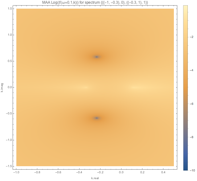
Fig. 1.117 MAA spectWC4 for \(\omega=0.1\).
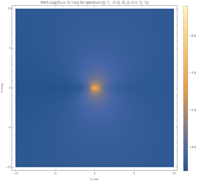
Fig. 1.118 MAA spectWC4 for \(\omega=-0.1\).
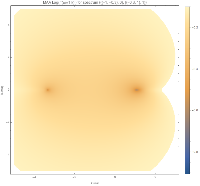
Fig. 1.119 MAA spectWC4 for \(\omega=-0.1\).
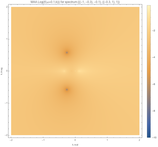
Fig. 1.120 MAA spectC1 for \(\omega=0.1\).
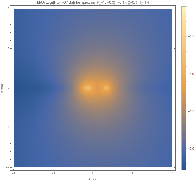
Fig. 1.121 MAA spectC1 for \(\omega=-0.1\).
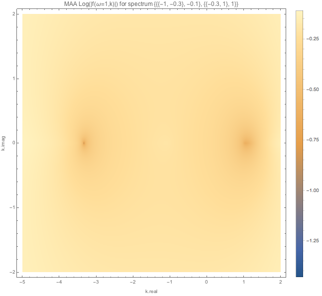
Fig. 1.122 MAA spectC1 for \(\omega=1\).
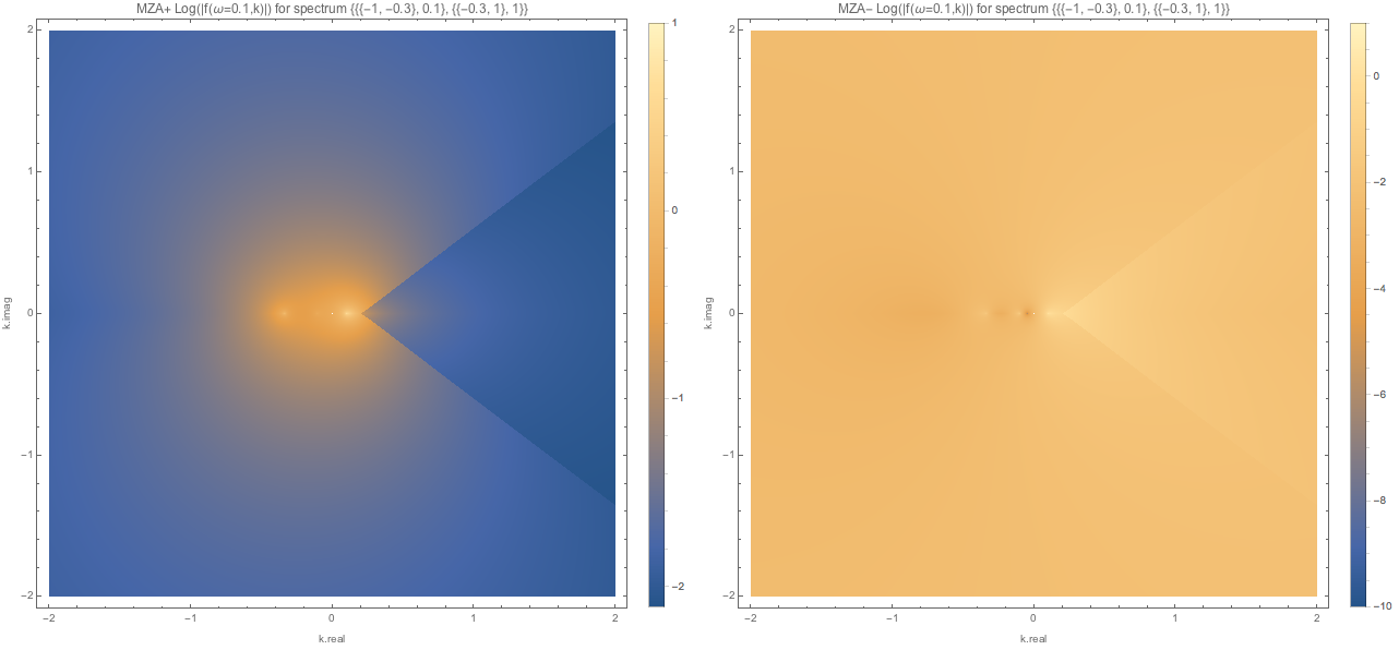
Fig. 1.123 MZA spectWC3 for \(\omega=0.1\).
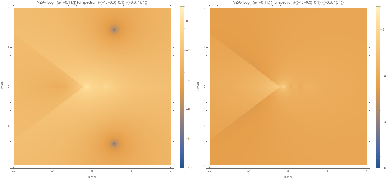
Fig. 1.124 MZA solution spectWC3 for \(\omega=-0.1\).
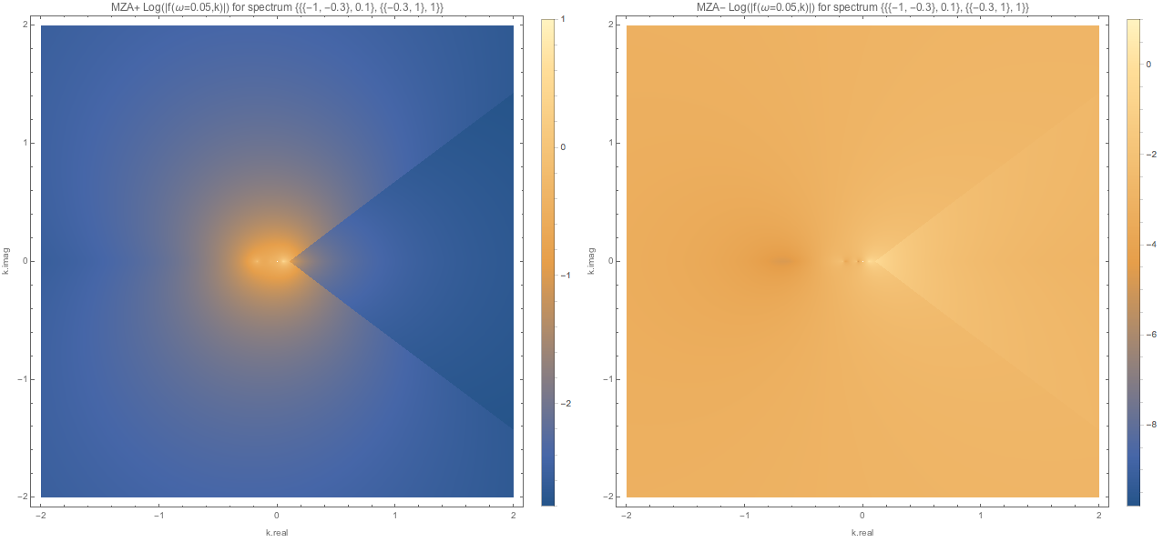
Fig. 1.125 MZA solutions spectWC3 for \(\omega=0.05\).
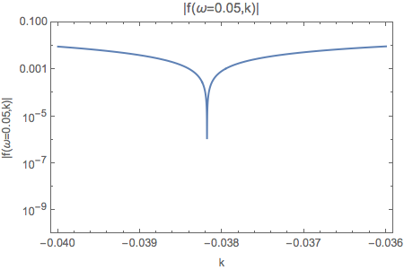
Fig. 1.126 MZA+ solution spectWC3 for \(\omega=0.05\) for a small range of \(k\). I chose only real \(k\).
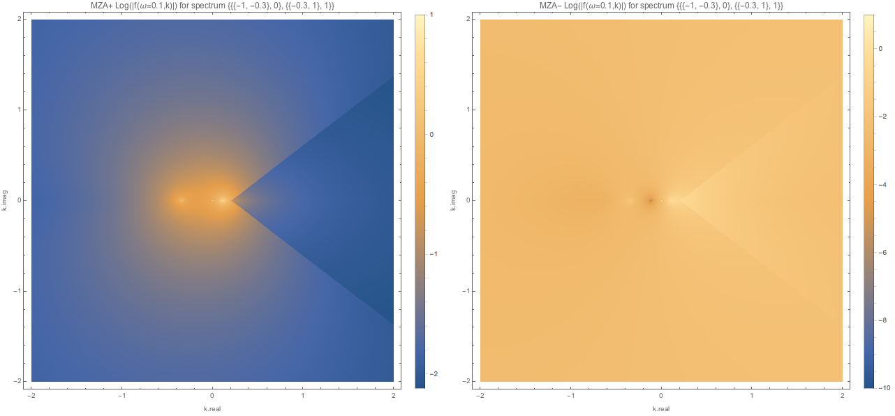
Fig. 1.127 MZA solution spectWC4 for \(\omega=0.1\).
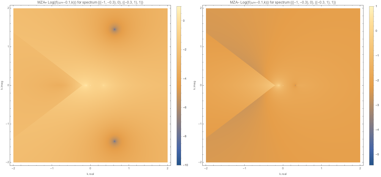
Fig. 1.128 MZA solution spectWC4 for \(\omega=-0.1\).

Fig. 1.129 MZA solution spectWC4 for \(\omega=0.05\).
Questions about MZA Solutions
The results are weird. For spectWC3 and spectWC4, no real solutions are found in DR for \(\omega=0.05\). However, here we found one real solution for \(k\), which is not 0.
MZA solutions for spectra with crossing are shown below.
Fig. 1.130 MZA solutions for spectC1 with \(\omega=0.1\)
Fig. 1.131 MZA solutions for spectC1 with \(\omega=-0.1\)
Fig. 1.132 MZA solutions for spectC1 with \(\omega=1\). We found one real solution for MZA- solution.
Fig. 1.133 MZA solutions for spectC1 with \(\omega=-1\). We found one real solution for MZA+ solution.
1.2.5.4. Instability Regions Stop at Axis \(\omega=0\) or \(k=0\)
Question about MZA solutions
It seems that we should Taylor expand around \(omega=0\) for MZA/MAA solutions to see what actually is happening. We can expand the \(I_m\)’s around small real \(\omega\), then perform the integral.
Can I do Taylor Expansion?
For discrete beams, we determine \(k\) using first order expansion of \(I_m\) at \(\omega\sim 0\).
We first look at MAA solution.
For generality we do not distingush between discrete beams and continuous beams. Instead, we define moments of spectrum to be
For MAA solutions, the equations we are interested in are
where
We perform Taylor expansion on \(\frac{u^m}{\omega - k u}\).
Eqn. (1.39) is simplified to
by dropping high orders. We are looking for solutions to this equation which is determined by the discriminant \(\Delta\).
The first term \((G_{-1}-G_1)^2\) is non-negative. I can tell that \(\omega\) plays a rule here. The question is how to quantify it.
Analatyically I could discuss the region of positive or negative \(\Delta\), i.e., real or imaginary solutions. But this is not simply determined by the sign of \(\omega\).
\(( G_{-2}-G_0 )>0\), \(\Delta<0\) requires \(\omega>\frac{ ( (G_{-1}-G_1)^2 }{ 16( G_{-2}-G_0 ) }\);
\(( G_{-2}-G_0 )<0\), \(\Delta<0\) requires \(\omega<\frac{ ( (G_{-1}-G_1)^2 }{ 16( G_{-2}-G_0 ) }\);
This is no really helpful and not correct.
From numerical calculations, we observe that \(\omega/k\to 0\), as \(\omega\to 0\). Thus we expect that
We investigate the behavior this solution around \(\omega\to 0\) so that the MAA solution simplifies to
We write down the real and imaginary part of the equation
where \(k = k_R + i k_I\). We are interested in imaginary part of \(k\) since it dertermines the instability. We rewrite the equation,
If \(G(0)\) is positive, we should have \(\omega>0\) to really have instabilities. And the value of imaginary part of \(k\) is fixed to \(\frac{G(0) \pi}{4}\) which is \(0.78\) if \(G(0)\)
MZA Solutions
For MZA solutions, I tried but it seems to be complicated. Neverthless I have the form of solutions. Need more thinking.
For MZA solutions, we have the equation
We calculate each terms at the limit \(\omega/k \to 0\).
\(1/k\) could be elimited on both sides. We define
Then the equation could be rewitten as
We seperate the imaginary part of the equation.
which is in fact
We solve \(k_I\).
Problems?
In principle we could solve \(k_R\) and \(k_I\) by combining both the real and imaginary part. However, the real part of the equation is quadratic in k.
I have the sign of \(\omega\) consistant with LSA for several spectra. But the numerical values are not exactly matching.
The problem of MZA- solutions becomes much more serious now.