1.5.1.2. 2017-04 Group Meeting
1.5.1.2.1. 2017-04-13
Show the new dispersion relations as well as the \(\omega(n)\) plots.
Crossing change the number of solutions for different n.
Ask about how to identify the plus and minus modes before the calculation in the 2013 paper: Duan, H. (2013). Flavor oscillation modes in dense neutrino media. Physical Review D - Particles, Fields, Gravitation and Cosmology, 88(12), 1–7.
1.5.1.2.2. 2017-04-19
The unstable points
1.5.1.2.2.1. Some Discussion on Scaling
Code
The corresponding Mathematica code is:
codebase.git/mma/linear-stability/growth-in-fourier-modes.nb
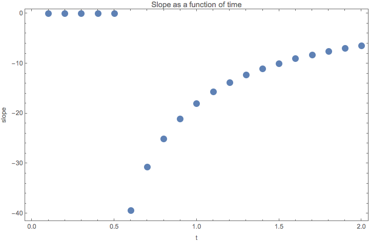
Fig. 1.191 Slope as a function of time. I tried log(-x) plot and it shows that -x decreases faster than exponential.
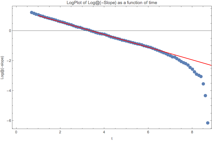
Fig. 1.192 In the beginning -x is decreasing as exp(exp(-k x + b)). But it than will be faster than this expression. The caveat is that the calculation of slope is not that accurate when it approaches 0. So we actually should truncate it. As being said, it might be a good idea to treat it as exp(exp(-k x + b)). The red line is \(1.48988 - 0.435439 x\).
This means that the time evolution of slope is quite complicated. But we should compare the slope at the same time for different parameters. For each time snapshot we should be able to guess the function of parameters that describes the slope.
As a very preliminary result, scale as I defined, changes how fast the perturbation is propagated into higher moments. So does the off diagonal element.
meh
The eigenvalues of this pseudo Hamiltonian
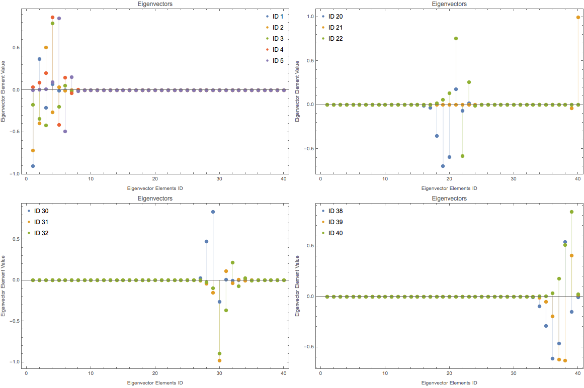
Fig. 1.193 Eigenvector components for different eigenvectors of this pseudo Hamiltonian. For mat[dim,1,1,1]
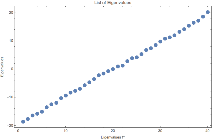
Fig. 1.194 Eigenvalues of this pseudo Hamiltonian. For mat[dim,1,1,1]
The key is actually the eigenvectors. If we assume each of the modes are plane waves, the eigenvalues are the ones that determines how fast the grow is while the eigenvectors tells us which element will grow. As I increase the scale, the eigenvectors seems to be more clean, i.e., fewer but hierarchial excited elements.
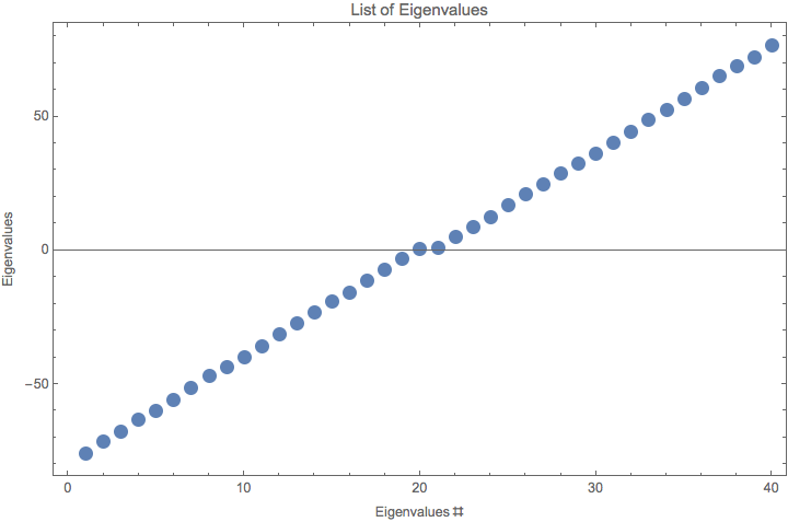
Fig. 1.195 Eigenvalues for mat[dim,4,1,1]. Notice that for the 20th and 21st eigenvalues are close to 0.
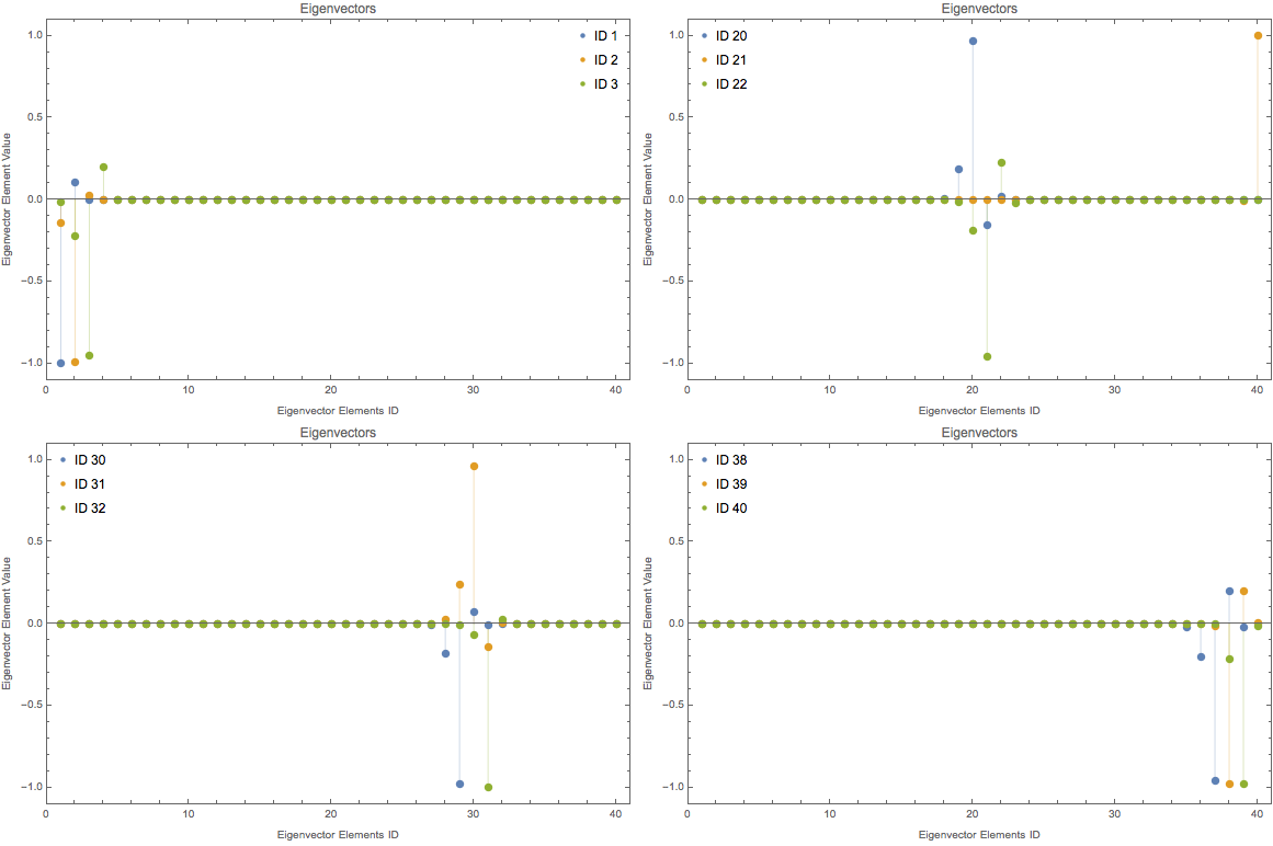
Fig. 1.196 Eigenvector components for different eigenvectors of this pseudo Hamiltonian. For mat[dim,4,1,1].
Decreasing the off diagonal elements have similar effect on eigenvectors which explains the similar structure of fourier modes for different off diagonal elements. However, they should have different growth rate as a function of time.
More explicitly, we plot out the logplot of eigenvector elements and we will see the exponential behavior.
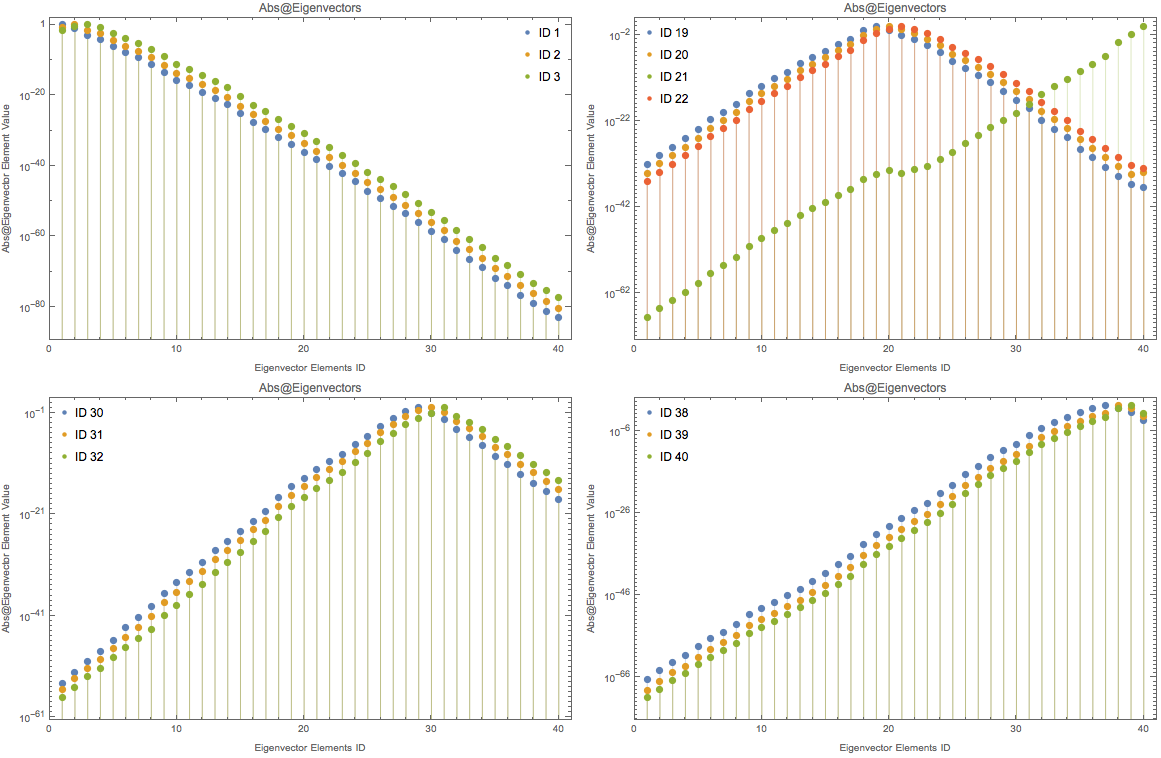
Fig. 1.197 LogPlot of Abs@eigenvecotors. For mat[dim,4,1,1].
Just for reference, the positive values of eigenvectors also have this exp behavior.
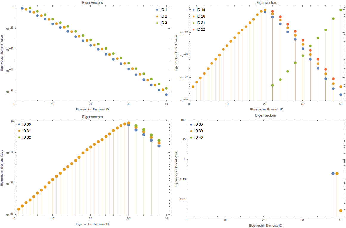
Fig. 1.198 LogPlot of positive elements of eigenvecotors. For mat[dim,4,1,1].
Do all the eigenvectors have the same slope?
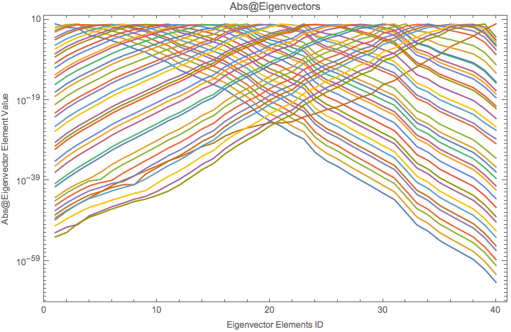
Fig. 1.199 All 40 eigenvectors for mat[dim,1,1,1]. Kind of same absolute values of slope.
Qualitatively we can see why the exponantial behavior in Fourier modes through the eigenvectors.
To guess an expression for it, I need to compare different scales.
As reference, we plot mat[dim,1,1,1].
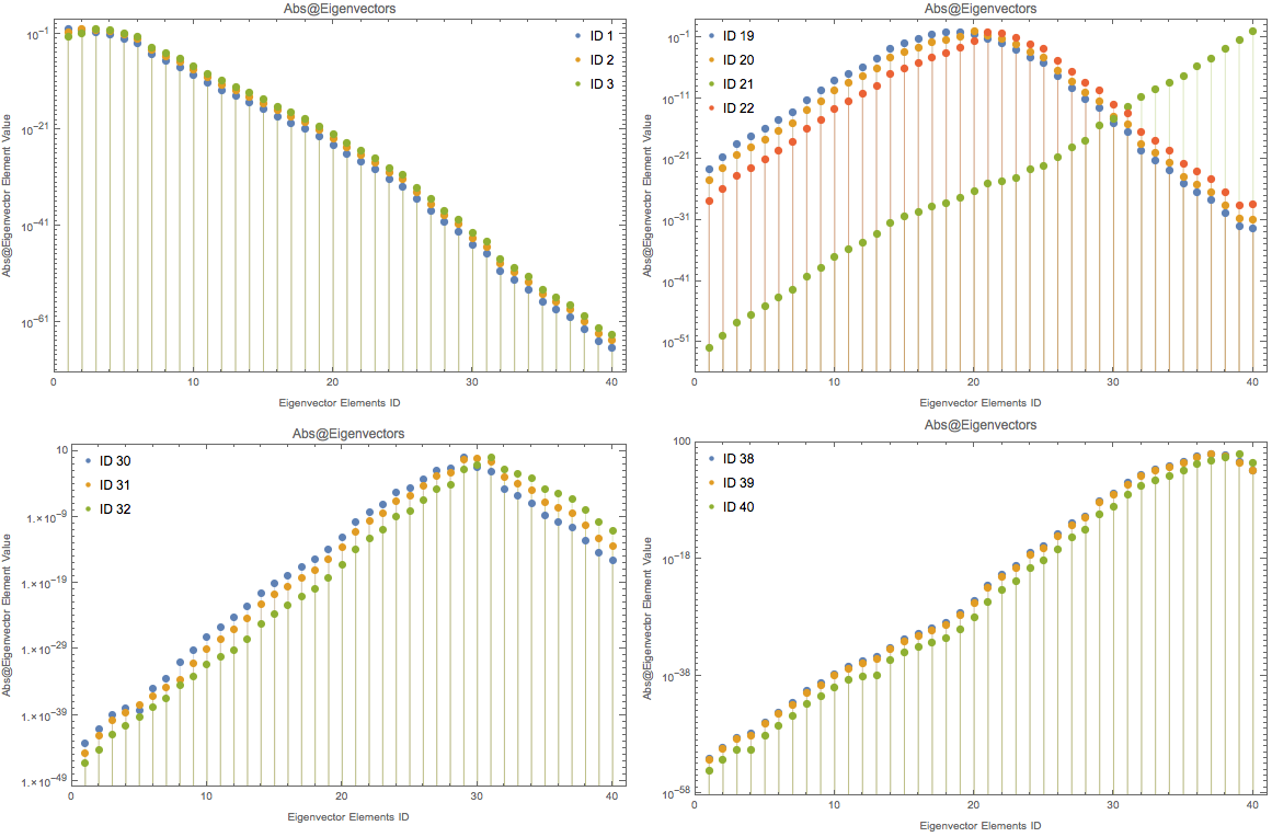
Fig. 1.200 LogPlot of Abs@eigenvecotors. For mat[dim,1,1,1].
Here is a plot that shows the slope of \(\text{Log@Abs@Eigenvalues}\sim \text{Eigenvalue Element ID}\).
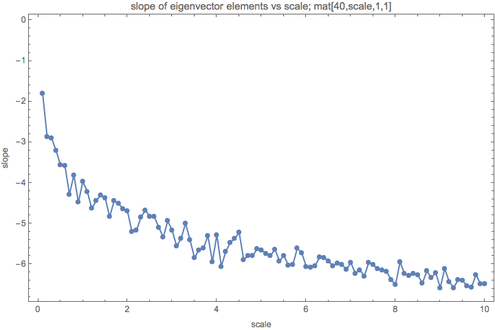
Fig. 1.201 Slope of eigenvector elements for different scales.
Ratio of Scale and Off diagonal?
Is the ratio of scale and off diagonal element responsible for the slope?
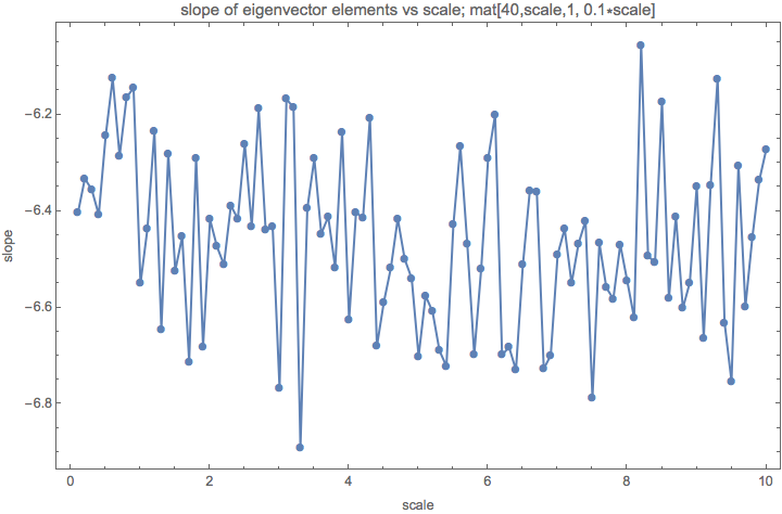
Fig. 1.202 The ratio of scales and off diagonal elements is roughly 10.
Or the plot with scale/off-diag = 1 to 10.
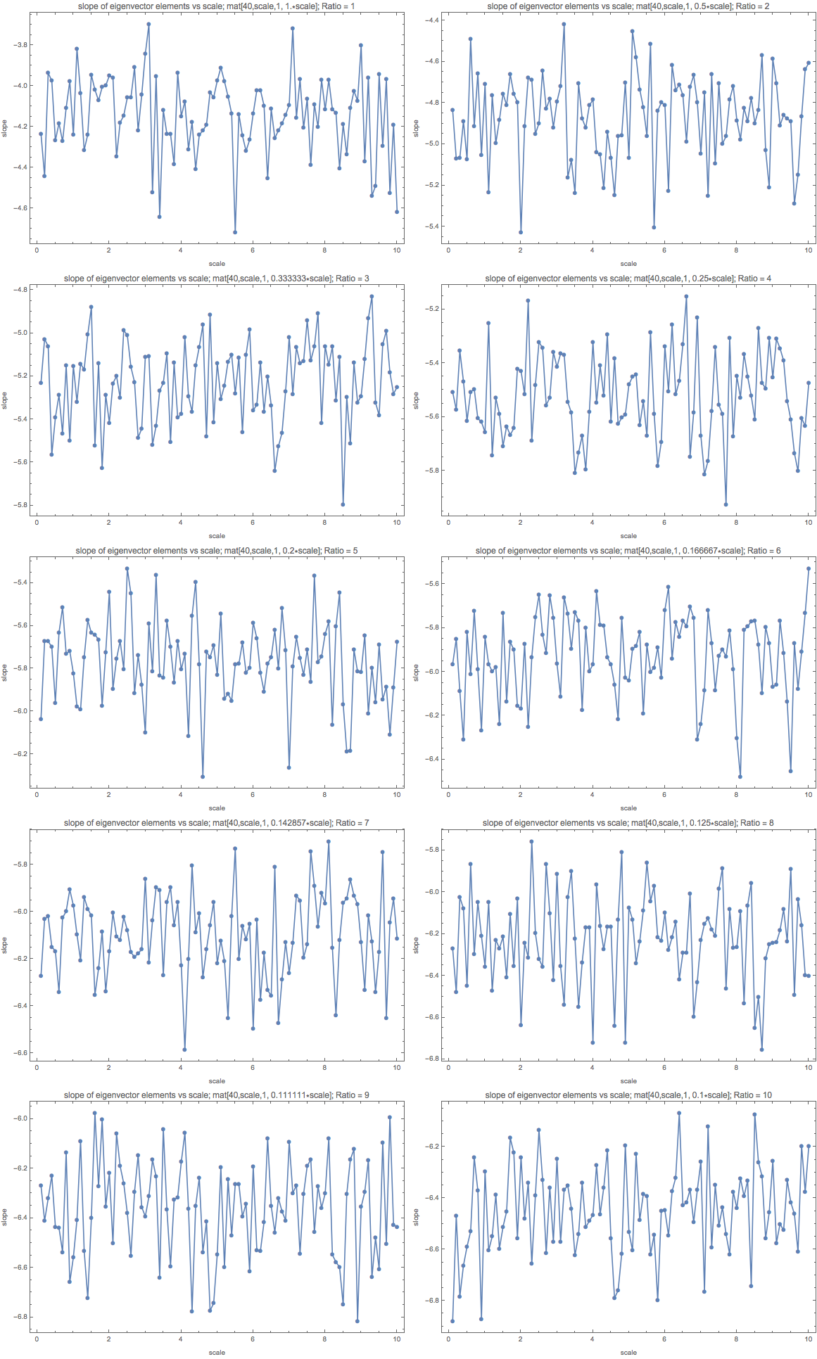
Fig. 1.203 The ratio of scales and off diagonal elements is roughly from 1 to 10. It almost matches the result from the calculation for different scales.
1.5.1.2.3. 2017-04-22
This is an update for the Fourier mode growth.
I recalculated the eigenvectors using a Hamiltonian without random numbers so that the Hamiltonian matrix is defined as
What I found is that if \(1/ratio = od/scale\) is small, the slope is related to the ration through
or in other words,
In the calculations I did, \(k\sim 1\).

Fig. 1.204 Slope vs Ratio
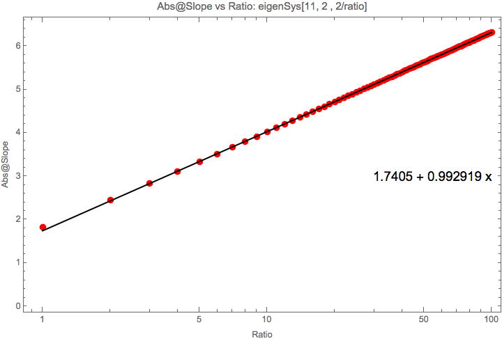
Fig. 1.205 Slope vs Ratio with scale = 2. The same as above thus the ratio is the key.
The dimension seems to change the interception.
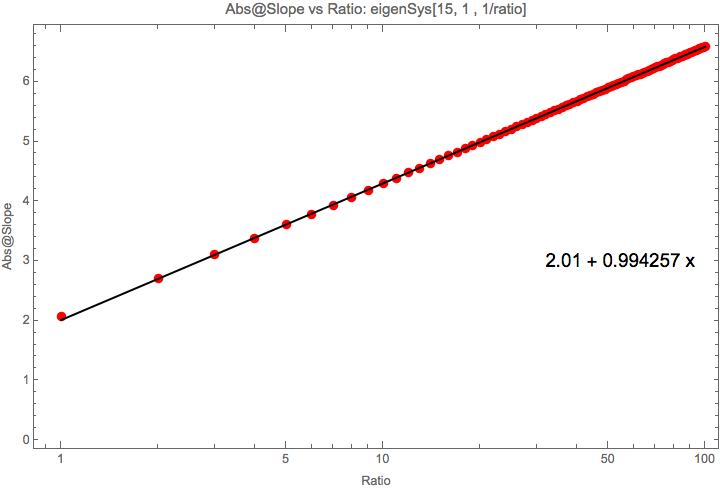
Fig. 1.206 Slope vs Ratio with dimension = 15.
Change the dimension seems to only slightly change the slope increasing rate.
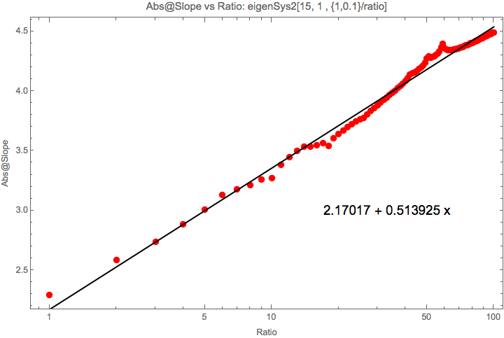
Fig. 1.207 Slope vs Ratio with pentadiag Hamiltonian.
Enough for these eigenvectors. To make a real connection with the time evolution or the long time limit of the time evolution, we need to find how the system evolves.
The idea is that all Fourier modes are oscillations. In the beginning of oscillations, it is simply a linear growth in time since Taylor expansion of \(e^{-i E t}\) is \(E t\).
Given an initial condition \(\psi(0)\) with only nonzero in the middle element, we can expand it using the eigenvectors \(\psi_i (0)\), i.e.,
What I find is that the coefficients \(A_i\) is actually a exponential shape.
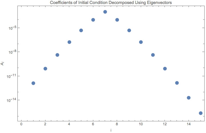
Fig. 1.208 logplot of coefficients \(A_i\).
If I start from all 1’s as initial condition, the evolution won’t be of this wedge shape and it will oscillation.
Fig. 1.209 Animation of value of each components of wave function, with inital condition all 1’s.
The corresponding decomposition of intial condition is shown in :numfig:`fourier-mode-growth-initial-all-1-decompose`.
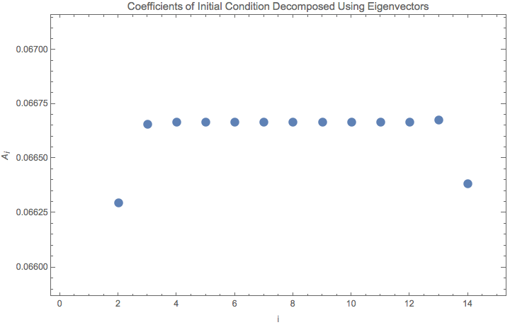
Fig. 1.210 logplot of coefficients \(A_i\).