1.1.8.1. Flavor Isospin AppliedUsing flavor isospin, the equation of motion is written as
\[\frac{d\vec s}{dx} = \vec{s} \times \vec H,\]
where
\[\begin{split}\vec s = \begin{pmatrix}
\mathrm{Re}(\psi_1^*\psi_2) \\
\mathrm{Im}(\psi_1^*\psi_2) \\
(\lvert \psi_1 \rvert^2 - \lvert \psi_2 \rvert^2)/2.
\end{pmatrix}\end{split}\]
Background Matter Basis
In background matter basis the Hamiltonian vector is
\[\begin{split}\vec H = \begin{pmatrix}
\delta \lambda(x) \sin 2\theta_m \\
0 \\
\omega_m - \delta \lambda(x) \cos 2\theta_m
\end{pmatrix}.\end{split}\]
For two perturbations, we write it as
\[\begin{split}\vec H = \begin{pmatrix}
0 \\
0 \\
\omega_m
\end{pmatrix} + \begin{pmatrix}
\delta \lambda_1(x) \sin 2\theta_m \\
0 \\
- \delta \lambda_1(x) \cos 2\theta_m
\end{pmatrix} + \begin{pmatrix}
\delta \lambda_2(x) \sin 2\theta_m \\
0 \\
- \delta \lambda_2(x) \cos 2\theta_m
\end{pmatrix}.\end{split}\]
The initial condition is
\[\begin{split}\Psi(0) = \begin{pmatrix}
1 \\
0
\end{pmatrix},\end{split}\]
which corresponds to a flavor isospin vector
\[\begin{split}\vec s(0) = \frac{1}{2} \begin{pmatrix}
0 \\
0 \\
1
\end{pmatrix}.\end{split}\]
T-basis
In this basis, the Hamiltonian is
\[\begin{split}H_1 &= -\frac{\omega_m}{2} \sigma_3 - \frac{\delta \lambda}{2} \sin 2\theta_m \begin{pmatrix}
0 & e^{2i\eta_1(x)} \\
e^{-2i\eta_1(x)} & 0
\end{pmatrix} \\
& = -\frac{\omega_m}{2} \sigma_3 +\frac{\delta \lambda}{2} \sin 2\theta_m \sin 2\eta_1(x) \sigma_2 - \frac{\delta \lambda}{2} \sin 2\theta_m \cos 2\eta_1(x) \sigma_1,\end{split}\]
or
\[\begin{split}H_2 &= - \frac{\delta \lambda}{2} \sin 2\theta_m \begin{pmatrix}
0 & e^{2i\eta_2(x)} \\
e^{-2i\eta_2(x)} & 0
\end{pmatrix} \\
&= \frac{\delta \lambda}{2} \sin 2\theta_m \sin 2\eta_2(x) \sigma_2 - \frac{\delta \lambda}{2} \sin 2\theta_m \cos 2\eta_2(x) \sigma_1,\end{split}\]
where the background is removed from diagonal elements in \(H_1\) but not in \(H_2\) .
The corresponding vectors are
\[\begin{split}\vec H_1 = \begin{pmatrix}
\delta\lambda \sin 2\theta_m \cos 2\eta_1(x) \\
-\delta\lambda \sin 2\theta_m \sin 2\eta_1(x)\\
\omega_m
\end{pmatrix},\end{split}\]
and
\[\begin{split}\vec H_2 = \begin{pmatrix}
\delta\lambda \sin 2\theta_m \cos 2\eta_2(x) \\
-\delta\lambda \sin 2\theta_m \sin 2\eta_2(x)\\
0
\end{pmatrix}.\end{split}\]
Given the initial condition in background matter basis
\[\begin{split}\Psi(0) = \begin{pmatrix}
1 \\
0
\end{pmatrix},\end{split}\]
we have to apply the T transformation to get the initial condition in the T-basis
\[\begin{split}\Psi_1(0) &= \begin{pmatrix} e^{i \eta_1 (x)} & 0 \\ 0 & e^{-i \eta_1 (x)} \end{pmatrix}\Psi(0) = \begin{pmatrix} e^{i \eta_1 (x)} \\ 0 \end{pmatrix} \\
\Psi_2(0) &= \begin{pmatrix} e^{i \eta_2 (x)} & 0 \\ 0 & e^{-i \eta_2 (x)} \end{pmatrix}\Psi(0) = \begin{pmatrix} e^{i \eta_2 (x)} \\ 0 \end{pmatrix},\end{split}\]
which correspond to flavor isospin vectors
\[\begin{split}\vec s_1(0) = \vec s_2(0) = \vec s(0) = \frac{1}{2} \begin{pmatrix}
0 \\
0 \\
1
\end{pmatrix},\end{split}\]
since the T transformation is unitary.
Modes
For each mode of the multi-frequency case, the Hamiltonian is
\[\begin{split}H = \frac{1}{2}\begin{pmatrix}
0 & B_N e^{i(n_i k_i -\omega_m)x} \\
B_N^* e^{-i(n_i k_i -\omega_m)x} & 0
\end{pmatrix},\end{split}\]
where \(B_N\) is either real or pure imaginary,
\[\begin{split}B_N &= -(-i)^{\sum_a n_a} \tan 2\theta_m \left( \sum_a n_a k_a \right) \left( \prod_a J_{n_a}\left( \frac{A_a}{k_a}\cos 2\theta_m \right) \right)\\
& = - \tan 2\theta_m \left( \sum_a n_a k_a \right) \left( \prod_a J_{n_a}\left( \frac{A_a}{k_a}\cos 2\theta_m \right) \right) e^{-i \sum_a n_a \pi/2}\\
& = \rho_{N} e^{-i \sum_a n_a \pi/2}.\end{split}\]
The Hamiltonian vector is
\[\begin{split}\vec H = \begin{pmatrix}
\rho_N \cos\left( (n_i k_i -\omega_m)x - \sum_a n_a \pi/2 \right) \\
-\rho_N \sin\left( (n_i k_i -\omega_m)x - \sum_a n_a \pi/2 \right) \\
0
\end{pmatrix}.\end{split}\]
1.1.8.2. Equilibrium Points, Linear Stability Analysis, and Limit CyclesIn background matter basis, the equation of motion is
\[\begin{split}\frac{d}{dx}\begin{pmatrix}
s_1 \\
s_2 \\
s_3
\end{pmatrix} = \begin{pmatrix}
s_1 \\
s_2 \\
s_3
\end{pmatrix} \times \begin{pmatrix}
\delta \lambda(x) \sin 2\theta_m \\
0 \\
\omega_m - \delta \lambda(x) \cos 2\theta_m
\end{pmatrix}.\end{split}\]
Such a system is still not easy to solve. However, we can use phase portrait to get some information.
The fixed points are obtained by setting \(\vec s\times \vec H = 0 = \frac{d}{dx}\vec s\) . Even though in general we need to obtain the fixed points first before infering the linear stability, this is not needed since this equation is linear to \(\vec s\) .
The Jacobian is obtained
\[\begin{split}J_{mn} & = \frac{d (\vec s\times \vec H)_m}{ds_n} \\
& = \begin{pmatrix}
0 & H_3 & -H_2\\
-H_3 & 0 & H_1 \\
H_2 & -H_1 & 0
\end{pmatrix},\end{split}\]
which comes from the result
\[\begin{split}\vec s\times \vec H = \begin{pmatrix}
s_2 H_3 - s_3 H_2 \\
s_3 H_1 - s_1 H_3 \\
s_1 H_2 - s_2 H_1
\end{pmatrix}.\end{split}\]
Plugin in the Hamiltonian in background matter basis, the eigenvalues of this Jacobian are
\[\begin{split}& 0 \\
& -\frac{1}{\sqrt{2}} \sqrt{ - ( A_1 \sin (k_1 x) -\omega_m )^2 + 2 A_1 \omega_m \sin (k_1 x) (1 - \cos 2\theta_m) }\\
& \frac{1}{\sqrt{2}} \sqrt{ - ( A_1 \sin (k_1 x) -\omega_m )^2 + 2 A_1 \omega_m \sin (k_1 x) (1 - \cos 2\theta_m) }.\end{split}\]
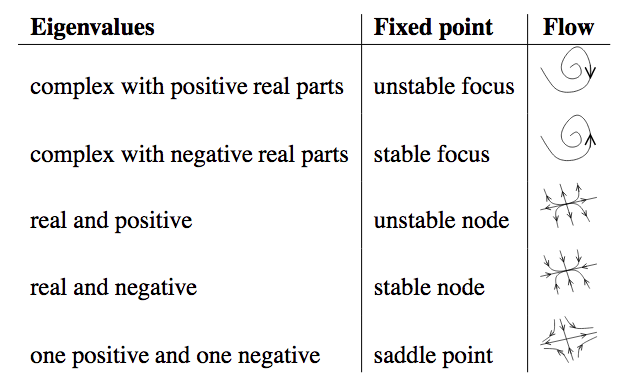
For \(- ( A_1 \sin (k_1 x) -\omega_m )^2 + 2 A_1 \omega_m \sin (k_1 x) (1 - \cos 2\theta_m) > 0\) , the eigenvalues have real parts, which means the system is a saddle point arround such equilibrium points.
Fig. 1.35 Eigenvalues of Jacobian and fixed points. Source: Stability Analysis for ODEs by Marc R. Roussel