1.1.7. Interference¶

Summary

Overall the system has at least two limits,

strong interference regime (the wavelength of the perturbations are of the same orders);
low-interference regime (one of the perturbations has a wavelength much larger than the others’).

For either case, the system is explained within the ralm of superpositions of multiple Rabi oscillations.

As for the first case, th criteria is related to both the resonance itself and the size of physical system we are interested in.

Each mode has an associated resonance, and explained by a single Rabi oscillation. Higher orders have much smaller resonance width than low orders.
Whether a mode is important to the system is determined by Q value, which is defined as the ratio of distance to resonance and resonance width.
However a mode with a wavelength that is much larger than the system is not counted since the resonance has not accumulated any significant transition probabilities within the region of the physical system.

However, we do not have a cystal clear understanding of such a strong interference.

The second case is essentially some limit of the strong interference. With Komogorov spectra of matter, the resonance is simplified in some sense. One of the limits is that one of the matter perturbations has much larger wavelength than the others, which will behave as a shift of the background matter density, within one wavelength of the small wavelength perturbations. Here we use two frequencies as examples, c.f. Fig. 1.27.

Even if the short wavelength one is exactly on resonance, adding the second perturbation as a background shift could move the system out of the resonance. The math behind it is related to the amplitude,

$\frac{{| B_{n} |}^{2}}{{| B_{n} |}^{2} + (n k - ω_{m})^{2}},$

where $n k - ω_{m} = 0$ for the resonance situation. As we add in the second long wavelength perturbation, $B_{n}$ , $ω_{m}$ will change. Nonetheless the relative change in $B_{n}$ is small while the change in $n k - ω_{m}$ is huge compared to $B_{n}$ value, if the amplitude of the new perturbation is large enough, i.e., $A_{2} ≫ | B_{n} |$ .
The caveat is that the wavelength of the second perturbation $k_{2}$ must be within a range much smaller than $k_{1}$ , and much larger than the resonance transition probability wavelength, roughly speaking, $k_{1} ≫ k_{2} ≫ | B_{n} |$ .
The newly added long wavelength merely has any effect when the system is in a region $\mod (k_{2} x, π) \sim 0$ , since $A_{2} \sin (k_{2} x) \sim 0$ for these values. Such regions probabily will appear multiple times within the size of physical system. Then we see accumulation effect, so that the transition amplitude will rise as we go furthure out.

From this point of view, the resonance is never destroyed since the accumulation will always be there.

In the calculation of multi-frequency matter background,

δ λ_{N} = \sum_{a = 1}^{N} A_{a} \sin (k_{a} x + ϕ_{a}),

we derived the equation of motion

i \partial_{x} Ψ = H Ψ,

where

\begin{array}{r} Ψ = (\begin{array}{c} ψ_{b 1} \\ ψ_{b 2} \end{array}), \end{array}

is the wave function in the T basis (new basis unitary transform from background matter basis using T matrix) and

\begin{array}{r} H = (\begin{array}{c} 0 & h_{N} \\ h_{N}^{*} & 0 \end{array}), \end{array}

where

h_{N} = - \frac{1}{2} \sum_{n_{1} = - \infty}^{\infty} \dots \sum_{n_{N} = - \infty}^{\infty} B_{N} Φ_{N} e^{i (\sum_{a}^{N} n_{a} k_{a} - ω_{m}) x},

and

\begin{aligned} B_{N} & = (- i)^{\sum_{a} n_{a}} (\sum_{a} n_{a} k_{a}) (\prod_{a} J_{n_{a}} (\frac{A_{a}}{k_{a}} \cos 2 θ_{m})), \\ Φ_{N} & = e^{i (\sum_{a} n_{a} ϕ_{a})} . \end{aligned}

1.1.7.1. Apply Approximations to Two Frequencies¶

We could identify the important combinations of n’s ${n_{1}, \dots, n_{N}}$ so that we can approximate the actual result.

The important question is combining multiple lists of n’s is not intuitively easy to understand. Here we consider the effect of adding new list of n’s to the system.

For simplicity a simplified system will be used,

\begin{array}{r} i \partial_{x} (\begin{array}{c} ψ_{b 1} \\ ψ_{b 2} \end{array}) = (\begin{array}{c} 0 & A_{1} e^{i ϕ_{1} x} + A_{2} e^{i ϕ_{2} x} \\ A_{1}^{*} e^{- i ϕ_{1} x} + A_{2}^{*} e^{- i ϕ_{2} x} & 0 \end{array}) (\begin{array}{c} ψ_{b 1} \\ ψ_{b 2} \end{array}) . \end{array}

Notice that $ϕ_{n}$ is always real but $A_{n}$ are either real or pure imaginary.

The matrix equation can be rewritten as systems of differential equations,

\begin{aligned} i \partial_{x} ψ_{b 1} & = (A_{1} e^{i ϕ_{1} x} + A_{2} e^{i ϕ_{2} x}) ψ_{b 2}, \\ i \partial_{x} ψ_{b 2} & = (A_{1}^{*} e^{- i ϕ_{1} x} + A_{2}^{*} e^{- i ϕ_{2} x}) ψ_{b 1} . \end{aligned}

This set of equations is solved by rewrite them to a second order differential equation

(1.26)¶

\partial_{x}^{2} ψ_{b 2} + \frac{A_{1}^{*} e^{- i ϕ_{1} x} + A_{2}^{*} e^{- i ϕ_{2} x})}{\partial_{x} (A_{1}^{*} e^{- i ϕ_{1} x} + A_{2}^{*} e^{- i ϕ_{2} x})} \partial_{x} ψ_{b 2} + (A_{1}^{*} e^{- i ϕ_{1} x} + A_{2}^{*} e^{- i ϕ_{2} x}) (A_{1} e^{i ϕ_{1} x} + A_{2} e^{i ϕ_{2} x}) ψ_{b 2} .

As a comparison, we also write down the equation for single n list,

\partial_{x}^{2} ψ_{b 2} + (\frac{i}{ϕ_{1}}) \partial_{x} ψ_{b 2} + | A_{1} |^{2} ψ_{b 2} = 0.

Approximations?

For single n list equation, the second term dominates if $ϕ_{1}$ is much smaller than 1. In the language of physics, the second term dominates if the system is very close to resonance.

$ϕ_{n}$ and resonance

$ϕ_{n}$ is in fact the deviation from exact resonance.

ϕ_{n} = \sum_{a}^{N} n_{a} k_{a} - ω_{m} .

In the multi-n-list case, this domination is easily destroyed. As an example, suppose we have $A_{1} = A_{2} = A$ and $ϕ_{2} = 10^{10} ϕ_{1}$ , the second term in equation (1.26) becomes

\frac{e^{- i ϕ_{1} x} + e^{- i 10^{10} ϕ_{1} x})}{\partial_{x} (e^{- i ϕ_{1} x} + e^{- i 10^{10} ϕ_{1} x})} \partial_{x} ψ_{b 2} = \frac{e^{- i ϕ_{1} x} + e^{- i 10^{10} ϕ_{1} x})}{(- i ϕ_{1} e^{- i ϕ_{1} x} - i 10^{10} ϕ_{1} e^{- i 10^{10} ϕ_{1} x})} \partial_{x} ψ_{b 2},

which can be dropped on as long as $ϕ_{1}$ is not as small as $10^{- 10}$ .

We exaggerated the situation.

1.1.7.2. Resonance Destroyed¶

1.1.7.2.1. General Ideas¶

We first investigate two frequencies. The Hamiltonian for a single frequency matter perturbation is

\begin{array}{r} \hat{H} = \sum_{n = - \infty}^{\infty} (\begin{array}{c} 0 & \frac{1}{2} {\hat{B}}_{n} e^{i (n \hat{k} - 1) \hat{x}} \\ \frac{1}{2} {\hat{B}}_{n}^{*} e^{- i (n \hat{k} - 1) \hat{x}} & 0 \end{array}), \end{array}

where

{\hat{B}}_{n} = (- i)^{n} \tan 2 θ_{m} n \hat{k} J_{n} (\frac{\hat{A}}{\hat{k}} \cos 2 θ_{m}) .

In some conditions, even we have on of the matter frequancy at resonance, this resonance could be destroyed when a new matter frequency is destroyed. Numerical calculations show that this could happen if the new perturbation is off resonance and with larger $B_{n_{2}}$ .

Let’s first set this first perturbation at resonance. Suppose we add in another matter perturbation with a frequency which is higher, i.e., $k_{2} ≪ k$ . Since the wavelength of this new perturbation is much larger, we will assume it doesn’t change within one wavelength of the first perturbation. Thus it behaves as an additional background. Will this new background destroy the resonance? Illustration of this idea is shown in Fig. 1.27.

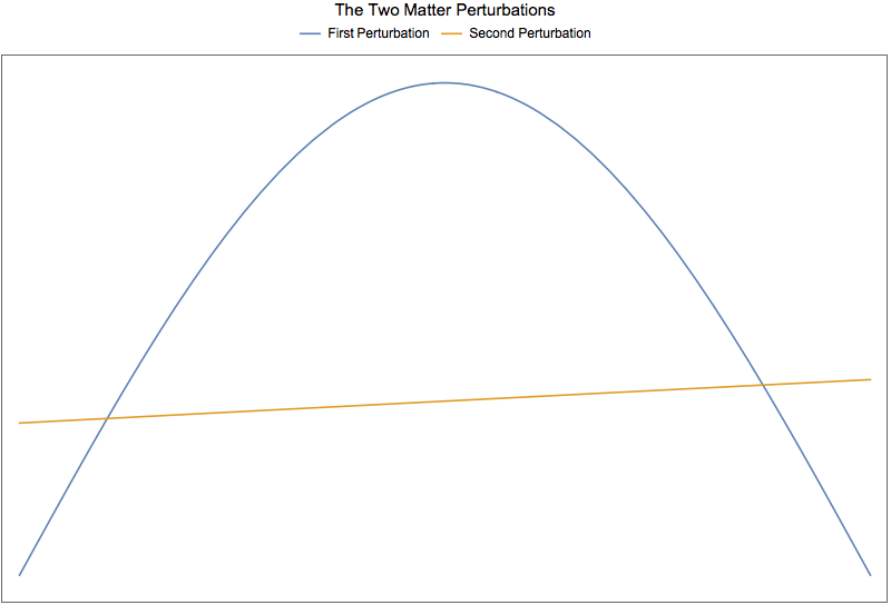
../../_images/second-freq-as-bg-illustration.png — Fig. 1.27 The two matter perturbations¶

To quantify this idea, we calculate the Q values for different modes with and without the new frequency. The procedure should be

Prepare the parameters: $ω_{v}$ , $λ_{0}$ (background matter profile), $λ_{1}$ (perturbation amplitude for first perturbation), $k_{1}$ (perturbation wavenumber for first perturbation)
Calculate the Q values.
Add in $λ_{2}$ (perturbation amplitude for the second perturbation) and treat this new perturbation as a constant within one wavelength of the first perturbation. Just use some random phase for the new matter profile, i.e., set $\sin (k_{2} x)$ to some resonanable value.
Recalculate the Q values.

Without the new perturbation (Mathematica Code):

deltamsquare13 = 2.6*10^(-15);(*MeV^2*)
energy20 = 20;(*Energy in units of MeV*)
thetaV = ArcSin[Sqrt[0.093]]/2
omegaVKK = OmegaVacuum[energy20, deltamsquare13](*MeV*)(*deltamsquare13/(2 energy20)(*MeV*)*)

lambdaNKK = 0.5*Cos[2 thetaV] omegaVKK (*MeV*)

onekListKK = {1};
oneaListKK =(*{0.1};*){0.02 (MeVInverse2km[ 2 Pi/(omegaMKK onekListKK[[1]])]/1500)^(5/3)};
onephiListKK = {0};

Part[qValueOrderdList[listNGenerator[1, 10], onekListKK, oneaListKK, onephiListKK, thetamV], 1 ;; 10];
Grid@%

which returns the Q value results for each modes:

{1}  0.
{-1} 577810.
{2}  1.75394*10^10
{-2} 5.26182*10^10
{3}  4.25927*10^15
{-3} 8.51854*10^15
{4}  1.16361*10^21
{-4} 1.93935*10^21
{5}  3.76761*10^26
{-5} 5.65142*10^26

Adding in the new frequency:

phi2 = Pi/2/100;

twoaListKK =(*{0.1,0.1};*){0.02 (MeVInverse2km[2 Pi/(omegaMKK*twokListKK[[1]])]/1500)^(5/3),
0.02 (MeVInverse2km[2 Pi/(omegaMKK twokListKK[[2]])]/1500)^(5/3)};

lambdaNKK2 = 0.5*Cos[2 thetaV] omegaVKK + Sin[phi2]*twoaListKK[[2]]*omegaMKK(*MeV*)

omegaMKK2 = OmegaMatter2[lambdaNKK2, thetaV, omegaVKK](*MeV*)
thetamV2 = Mod[ArcTan[Sin[2 thetaV]/(Cos[2 thetaV] - (lambdaNKK2/omegaVKK)^2)]/2, Pi]

onekListKK2 = {1}*omegaMKK/omegaMKK2;
oneaListKK2 =(*{0.1};*){0.02 (MeVInverse2km[2 Pi/(omegaMKK2 onekListKK2[[1]])]/1500)^(5/3)};

Part[qValueOrderdList[listNGenerator[1, 10], onekListKK2, oneaListKK2, onephiListKK, thetamV2], 1 ;; 10]
Grid@%

and the results for Q values of different modes are:

{1}  246.833
{-1} 577687.
{2}  1.75752*10^10
{-2} 5.26655*10^10
{3}  4.27026*10^15
{-3} 8.53505*10^15
{4}  1.16758*10^21
{-4} 1.94507*10^21
{5}  3.78384*10^26
{-5} 5.67375*10^26

The corresponding plots are shown in Fig. 1.28 and Fig. 1.29

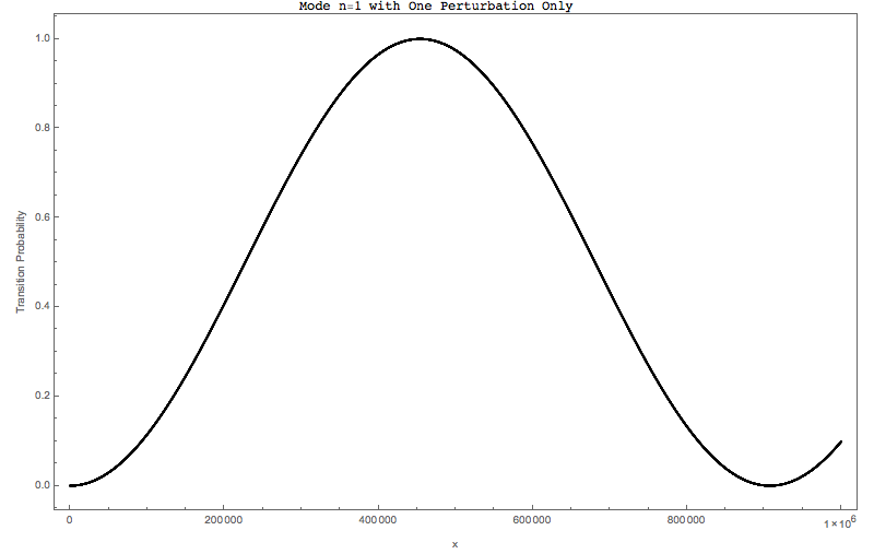
../../_images/second-freq-as-bg-example-1-first-freq-only.png — Fig. 1.28 Only the first frequency which is at resonance¶

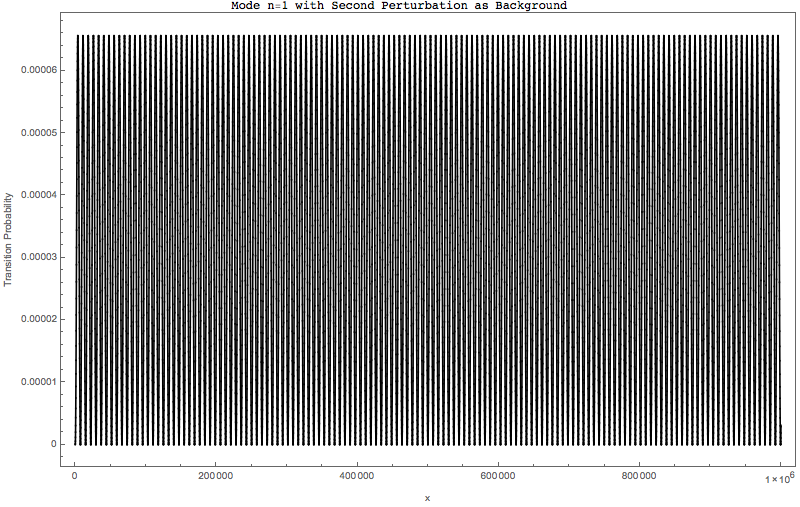
../../_images/second-freq-as-bg-example-1-with-second-freq-as-bg.png — Fig. 1.29 With the second frequency added in but only as a shift in background density¶

What determines the amplitude is

\frac{{| B_{n} |}^{2}}{{| B_{n} |}^{2} + (n k - ω_{m})^{2}} .

In this example, the coefficient in unit of $ω_{m}$ for one perturbation only is

| B_{1} | = 3.46135 \times 10^{- 6},

while it shifts a little bit when the second frequency is added in as a background shift, in unit of $ω_{m}$ ,

| B_{1}^{'} | = 3.46356 \times 10^{- 6} .

We set the first frequency at resonance, which means

k - ω_{m} = 0.

With the apprearance of the second frequency, what we have now is, in unit of $ω_{m}$ ,

k - ω_{m}^{'} = 0.000854192,

which is far beyond the width of the resonance.

1.1.7.2.2. Some Artifical Systems¶

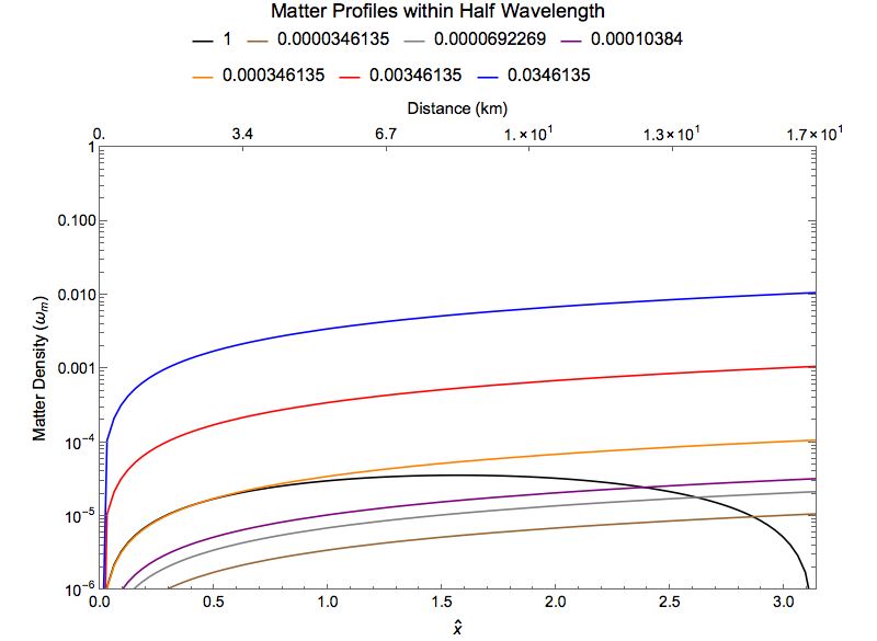
../../_images/second-freq-as-bg-1-divided-10-10-20-30-100-1000-10000-matter-density.png — Fig. 1.30 Matter profiles with one wavelength of the first perturbation¶

The resonance from the first perturbation is destroyed as the second perturbation grows much larger than it.

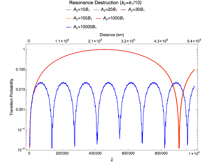
../../_images/second-freq-as-bg-1-divided-10-10-20-30-100-1000-10000-full-numerical.png — Fig. 1.31 Full numerical solutions¶

The hint is, the shift of the background matter profile is related to the destruction effect, whether it’s true destruction or effective destruction (destruction within a region).

An investigation of the most important mode shows that it is destroyed due to the a shift of background matter density.

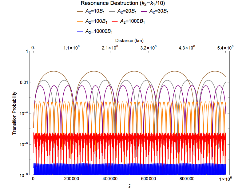
../../_images/second-freq-as-bg-1-divided-10-10-20-30-100-1000-10000-log.png — Fig. 1.32 Resonance destruction of the first mode¶

To verify how the interference actually works, we plot the full numerical calculation and the {1,0} mode, for comparision

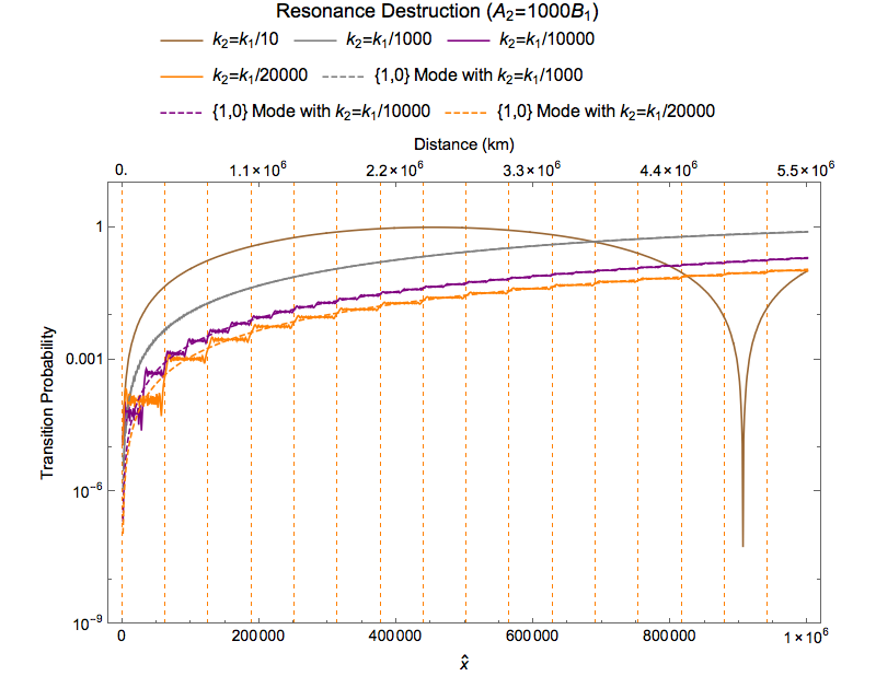
../../_images/second-freq-as-bg-1-d-10-1-d-1000-1-d-10000-1-d-200000-1000-full-numerical-with-10-mode-with-gridlines.png — Fig. 1.33 The solid lines are the full numerical calculations of the system; Dashed lines are {1,0} mode of the corresponding parameters; Vertical grid lines are the positions of zero amplitudes of the second matter perturbation.¶

It is clearly shown in Fig. 1.33 that each vicinity of zero amplitude for the second perturbation, the transition amplitude will increase, due to the resonance of the first perturbation.

What’s more interesting is that as $A_{2}$ becomes much larger than $A_{1}$ , the resonance seams to be destroyed. As an example, here we take $A_{2} = 0.0346135, A_{1} = 0.0000357347$ both in unit of $ω_{m}$ , which means $A_{2}$ is almost three orders larger than $A_{1}$ . The results are shown in Fig. 1.34.

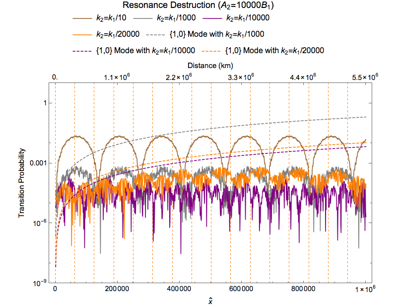
../../_images/second-freq-as-bg-1-d-10-1-d-1000-1-d-10000-1-d-200000-10000-full-numerical-with-10-mode-with-gridlines.png — Fig. 1.34 The solid lines are the full numerical calculations of the system; Dashed lines are {1,0} mode of the corresponding parameters; Vertical grid lines are the positions of zero amplitudes of the second matter perturbation.¶

1.1.7. Interference¶

1.1.7.1. Apply Approximations to Two Frequencies¶

1.1.7.2. Resonance Destroyed¶

1.1.7.2.1. General Ideas¶

1.1.7.2.2. Some Artifical Systems¶

1.1.7.3. Refs & Notes¶