1.1.6. Multi-frequency¶

1.1.6.1. 3 Frequencies¶

To extend what we have done to more frequencies is easy. For 3 frequencies, the 12 element of Hamiltonian has such a pattern that

\[\begin{split}h &= {\color{blue} \delta \lambda_1 \sum_{n_1} \cdots } {\color{red} \sum_{n_2} \cdots } {\color{cyan}\sum_{n_3} \cdots } + {\color{blue}\sum_{n_1} \cdots } {\color{red} \delta \lambda_2 \sum_{n_2} \cdots } {\color{cyan}\sum_{n_3} \cdots } + {\color{blue}\sum_{n_1} \cdots } {\color{red} \sum_{n_2} \cdots } {\color{cyan} \delta \lambda_3 \sum_{n_3} \cdots } \\ & \equiv h_1 + h_2 + h_3.\end{split}\]

Split Hamiltonian Strategy

As what we have tried in 2-frequency case, these terms can be viewed as three terms each is the interference between one frequency and the other two.

First of all, we assume the most important terms for \(h_1,h_2,h_3\) are determined by the \(k_1,k_2,k_3\) alone resonance respectively. Then we need to explore which terms to keep in the other two summations. Since the other two summations in each term are symmetric, we would like to include the resonance condition for one of them.

As an example, the first assumption leads to

\[h_1 \approx {\color{blue} \delta \lambda_1 \cdots(with n_{1,0} in it) } {\color{red} \sum_{n_2} \cdots } {\color{cyan}\sum_{n_3} \cdots }.\]

Then we include the other resonances.

A simple test using Mathematica shows that it doesn’t work.

We continue to rewrite the Hamiltonian by combining all terms. First of all, we write down the general form of Hamiltonian 12 element for \(N\) frequencies which is similar to Hamiltonian of two frequency case,

\[h = \frac{\sin 2\theta_m}{2}\sum_{a=1}^{N}A_a\sin(k_a x + \phi_a) e^{-i\omega_m x} \Pi_{a_1}^N \sum_{n_a=-\infty}^{\infty} (-i)^{n_a} J_{n_a}(\frac{A_a}{k_a}\cos 2\theta_m) e^{i n_a ( k_a x + \phi_a)} .\]

For three frequency perturbation,

\[h &= \frac{\sin 2\theta_m}{4i}\sum_{a=1}^{3}A_a( e^{i(k_a x + \phi_a - \omega_m x)} - e^{-i(k_a x + \phi_a + \omega_m x)} ) \Pi_{a_1}^N \sum_{n_a=-\infty}^{\infty} (-i)^{n_a} J_{n_a}(\frac{A_a}{k_a}\cos 2\theta_m) e^{i n_a ( k_a x + \phi_a)} .\]

Elaborate more on the math, we have (need a verification for this result)

\[h = \frac{1}{2}\sum_{n_1=-\infty}^\infty \sum_{n_2=-\infty}^\infty \sum_{n_2=-\infty}^\infty \left( B_{3,1} + B_{3,2} + B_{3,3} \right) \Phi_3 e^{i(n_1 k_1 +n_2 k_2 + n_3 k_3 -\omega_m)x},\]

where

\[\begin{split}B_{3,1} &= - (-i)^{n_1+n_2+n_3} \tan 2\theta_m n_1 k_1 J_{n_1}(\frac{A_1}{k_1}\cos 2\theta_m)J_{n_2}(\frac{A_2}{k_2}\cos 2\theta_m)J_{n_3}(\frac{A_3}{k_3}\cos 2\theta_m) \\ B_{3,2} & = - (-i)^{n_1+n_2+n_3} \tan 2\theta_m n_2 k_2 J_{n_1}(\frac{A_1}{k_1}\cos 2\theta_m)J_{n_2}(\frac{A_2}{k_2}\cos 2\theta_m)J_{n_3}(\frac{A_3}{k_3}\cos 2\theta_m) \\ B_{3,3} & = - (-i)^{n_1+n_2+n_3} \tan 2\theta_m n_3 k_3 J_{n_1}(\frac{A_1}{k_1}\cos 2\theta_m)J_{n_2}(\frac{A_2}{k_2}\cos 2\theta_m)J_{n_3}(\frac{A_3}{k_3}\cos 2\theta_m)\\ \Phi &= e^{i(n_1\phi_1 + n_2\phi_2+n_3\phi_3)}.\end{split}\]

In other words,

\[h = - \frac{1}{2}\sum_{n_1=-\infty}^\infty \sum_{n_2=-\infty}^\infty \sum_{n_2=-\infty}^\infty (-i)^{n_1+n_2+n_3} \left( n_1 k_1 + n_2 k_2 + n_3 k_3 \right) J_{n_1}(\frac{A_1}{k_1}\cos 2\theta_m)J_{n_2}(\frac{A_2}{k_2}\cos 2\theta_m)J_{n_3}(\frac{A_3}{k_3}\cos 2\theta_m) \Phi_3 e^{i(n_1 k_1 +n_2 k_2 + n_3 k_3 -\omega_m)x}.\]

Are 2 Frequencies Enough to Solve 3 Frequency Problems

We could try to use two frequencies to approach the actual 3 frequency problem first. To see the result, we first need to solve 3 frequency problem numerically without any approximation.

Then we choose pairs of integers to approach the 3 frequency system.

An calculations shows that this is not generally true, even though sometimes it is.

1.1.6.2. N Frequencies¶

Given a system with N perturbations

\[\delta\lambda_N = \sum_{a=1}^N A_a \sin(k_a x + \phi_a),\]

the Hamiltonian can be written as

\[\begin{split}H = \begin{pmatrix} 0 & h_N \\ h_N^* & 0 \end{pmatrix},\end{split}\]

where the Hamiltonian 12 element is

\[h_N = \frac{1}{2}\sum_{n_1=-\infty}^\infty \cdots \sum_{n_N=-\infty}^\infty B_N\Phi_N e^{i(\sum_a n_a k_a - \omega_m)x},\]

where

\[\begin{split}B_N &= -(-i)^{\sum_a n_a} \tan 2\theta_m \left( \sum_a n_a k_a \right) \left( \prod_a J_{n_a}\left( \frac{A_a}{k_a}\cos 2\theta_m \right) \right),\\ \Phi_N &= e^{i\left( \sum_a n_a \phi_a \right)}.\end{split}\]

It might be useful to notice that \((-i)^{\sum_a n_a} = (e^{-i \pi/2})^{\sum_a n_a} = e^{-i \pi\sum_a n_a/2}\). Such an phase won’t change the final transition probability given the initial condition that the system is completely on the low energy state.

To do

To actually make some sense here. I need to find out which approximation breaks down in Kelly’s paper; Ref to admonition Which Approximation Breaks Down. Check!
Use physical length scales to simplify/obscure the problem. Check!
How can small \(k\) destroy the resonance of large \(k\)? c.f., Kelly’s PRD paper.

1.1.6.3. Numerical Results¶

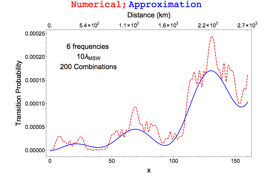
For an example system with 6 frequencies, with background matter profile \(\lambda=10\lambda_{\mathrm{MSW}}=10\cos(2\theta_v)\omega_v\), \(\sin 2\theta_v = 0.093\), \(\delta m^2 = \delta m_{13}^2=2.6\times 10^{-15}\), energy \(10\mathrm{MeV}\)

\[\hat k = \{2.6138748783741892734981263895723814892738971298790875814789472389461\\]

29836741984650871234, 1.8, 1.4, 0.9, 0.7, 0.3}

and perturbation amplitudes

\[\hat a = 0.1\hat k^{-5/3} = \{0.0201616, 0.0375445, 0.057076, 0.119196, 0.181205, 0.743814\}.\]

Fig. 1.26 Matter profile with 6 frequencies¶